Method 1 – Using ‘Text that Contains’ Option for Highlighting Partial Text Matches
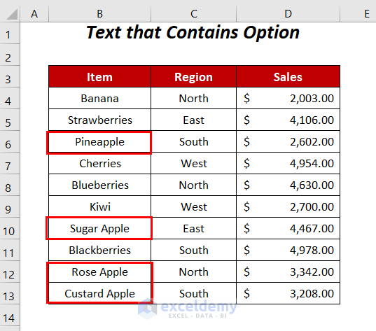
In the sample dataset, we will highlight cells that contain the text Apple such as Pineapple, Sugar Apple, Rose Apple, and Custard Apple .
Steps:
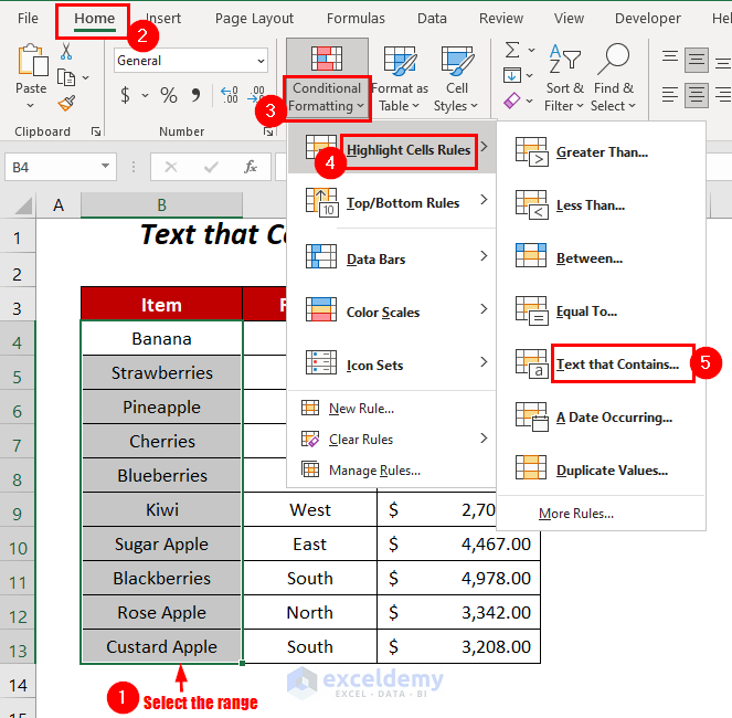
➤ Select the range and go to the Home tab >> Styles Group >> Conditional Formatting Dropdown >> Highlight Cells Rules Option >> Text that Contains… Option.
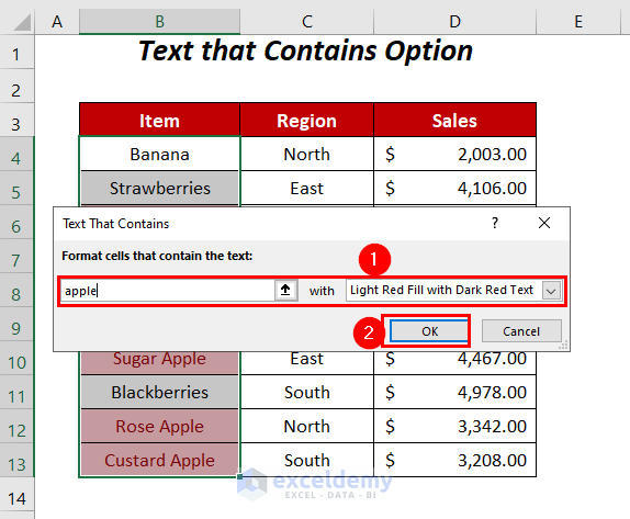
The Text That Contains dialog box will open.
➤ Enter apple in the first box and select the formatting style (here, Light Red Fill with Dark Red Text style has been selected) in the second box.
➤ Press OK.
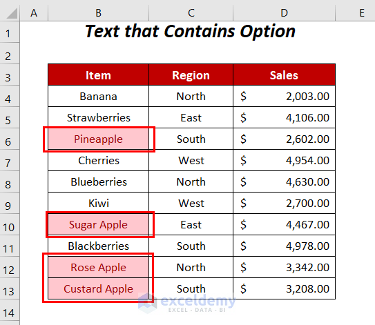
Conditional Formatting will be applied to the cells of the Item column having a partial match with Apple or apple.
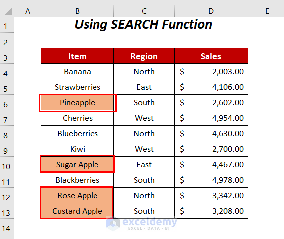
Method 2 – Using SEARCH Function
Step 1:
➤ Select the range and go to the Home tab >> Styles Group >> Conditional Formatting Dropdown >> New Rule Option.
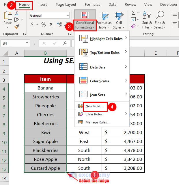
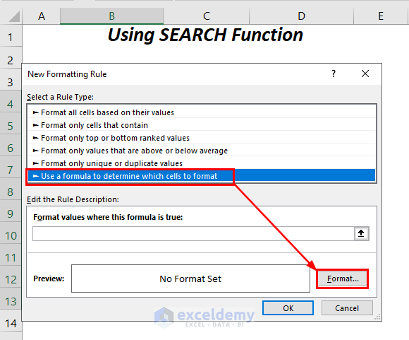
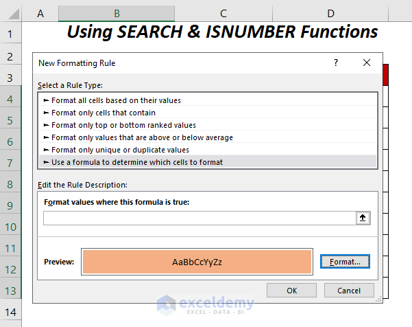
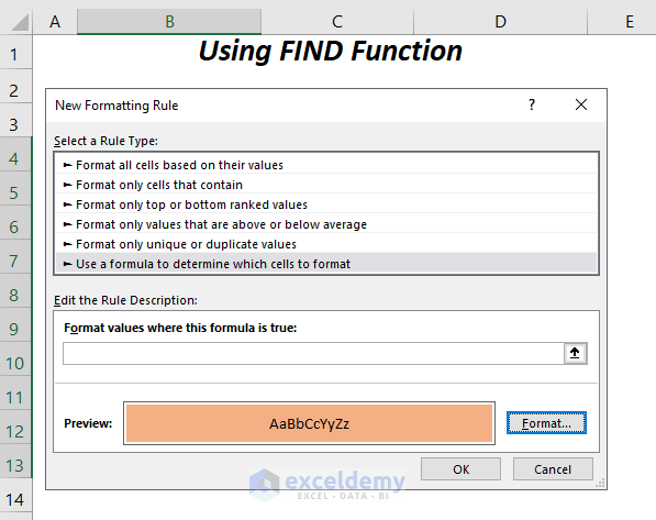
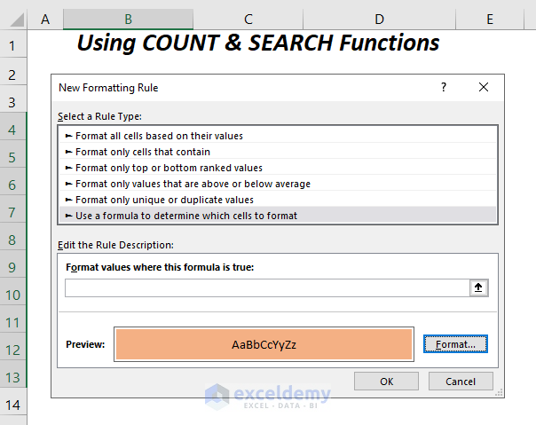
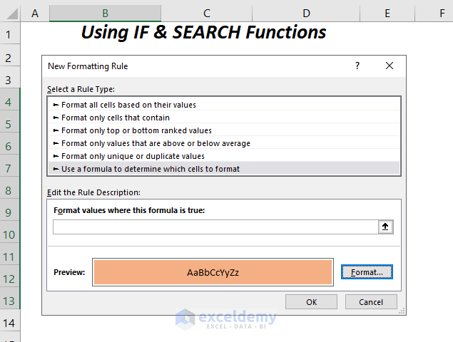
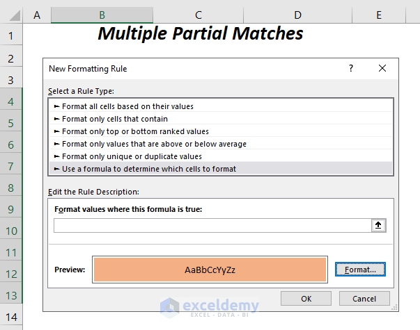
The New Formatting Rule wizard will open.
➤ Select Use a formula to determine which cells to format and click on Format.
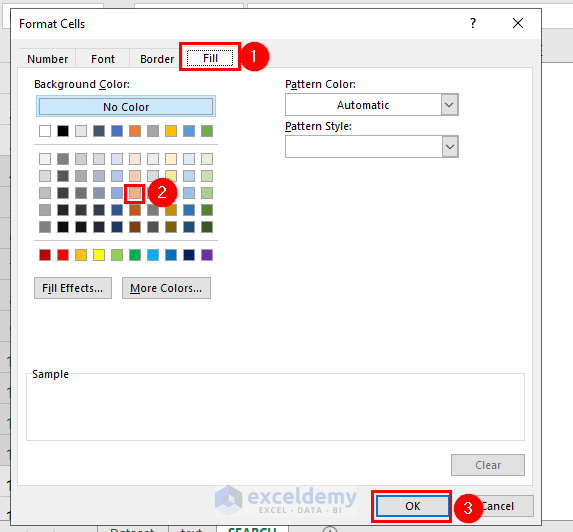
The Format Cells dialog box will open.
➤ Select the Fill Option and choose any Background Color. Click OK.
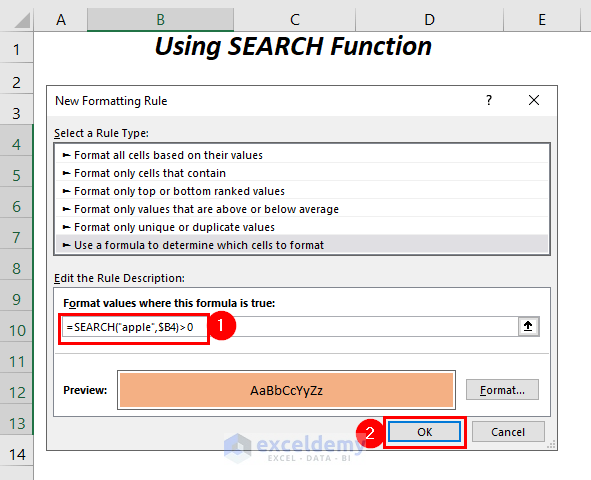
The New Formatting Rule dialog box will open.

Step 2:
➤ Add the following formula in the Format values where this formula is true box
=SEARCH("apple",$B4)>0SEARCH will look for the portion apple in the cells of Column B and for finding any matches it will return a value which will be the starting position of the apple in the full text and so for finding the matches, it will return a value greater than 0.
➤ Press OK.
The cells containing a partial match with Apple or apple will be highlighted.
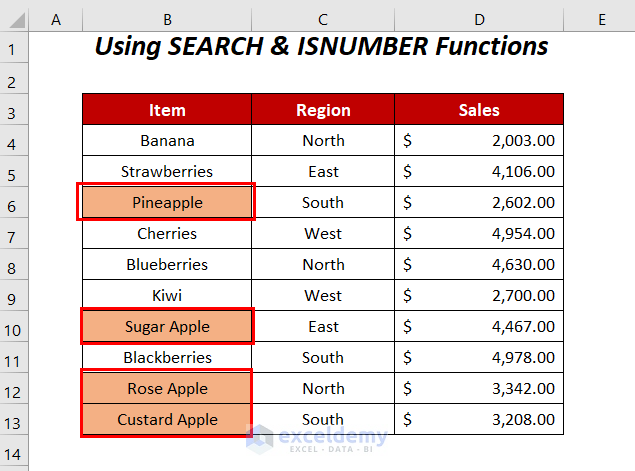
Method 3 – Using SEARCH and ISNUMBER Functions
Steps:
➤ Follow Step 1 of Method 2.
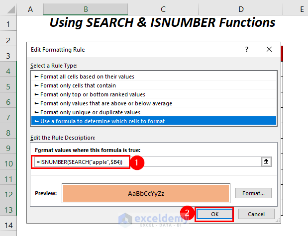
➤ Add the following formula in the Format values where this formula is true box
=ISNUMBER(SEARCH("apple",$B4))SEARCH will look for the portion apple in the cells of Column B and for finding any matches it will return a value which will be the starting position of the apple in the full text. And so ISNUMBER will return a TRUE if it gets any numeric value otherwise FALSE.
➤ Press OK.
Conditional Formatting will be applied to the cells that have a part of the whole text as Apple or apple.
Method 4 – Conditional Formatting for Case-Sensitive Partial Text Match Using FIND Function
Steps:
➤ Follow Step 1 of Method 2.
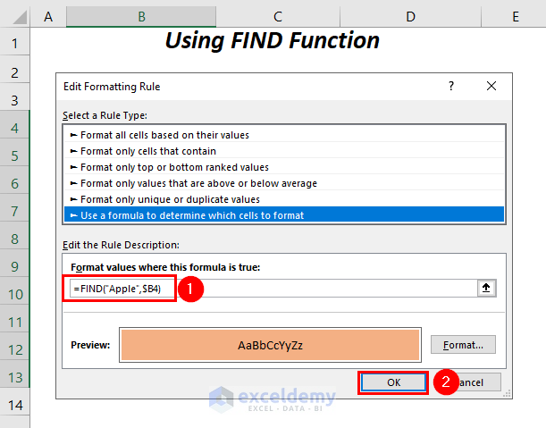
➤ Add the following formula in the Format values where this formula is true box
=FIND("Apple",$B4)FIND will look for the portion Apple in the cells of Column B and for finding any matches it will return a value which will be the starting position of the Apple in the full text. For not matching with the cases of Apple properly, we will not get any value.
➤ Press OK.
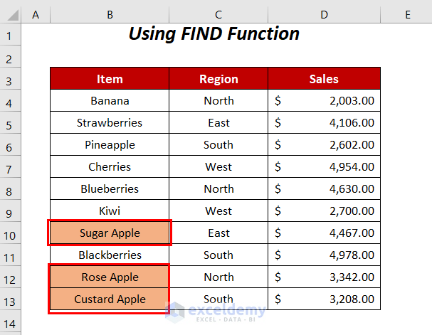
The cells of the Item column having the texts Sugar Apple, Rose Apple and Custard Apple will be highlighted.
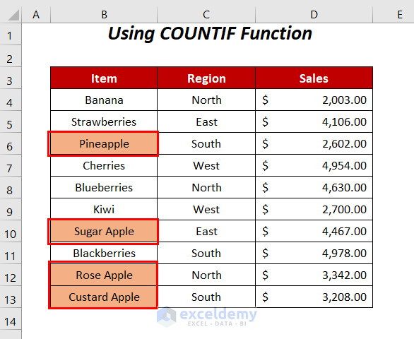
Method 5 – Using COUNTIF Function for Checking Partial Text Match
Steps:
➤ Follow Step 1 of Method 2.
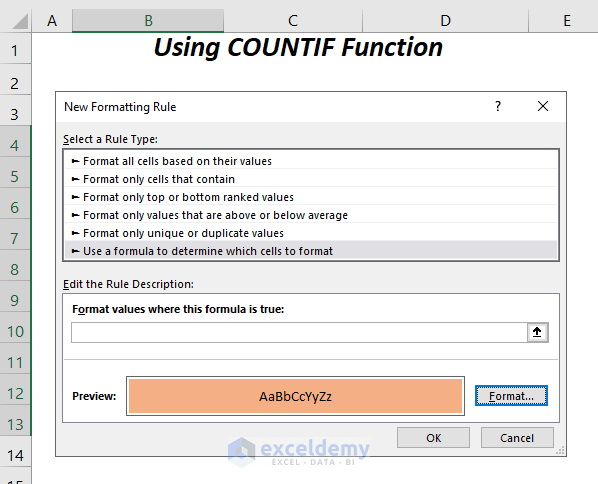
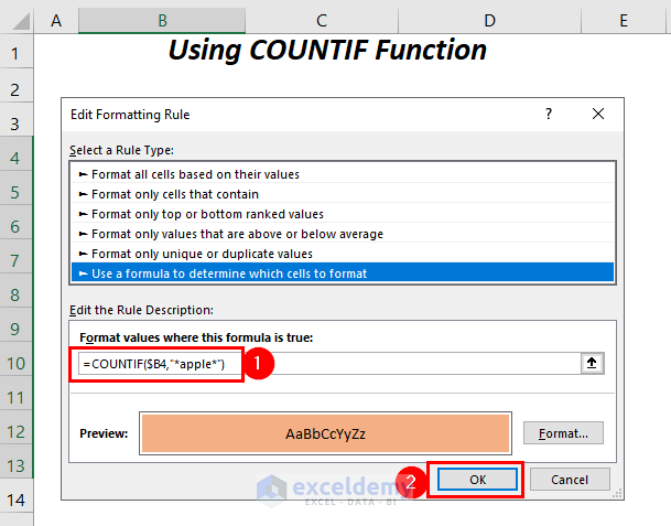
➤ Add the following formula in the Format values where this formula is true box
=COUNTIF($B4,"*apple*")By using the wildcard symbol * before and after apple we are ensuring the partial matches here and COUNTIF will return the number of times this text portion appears in the cells of Column B.
➤ Press OK.
Conditional Formatting will be applied to the cells having a portion of Apple or apple in the Item column.
Method 6 – Using Combination of COUNT and SEARCH Functions
Steps:
➤ Follow Step 1 of Method 2.
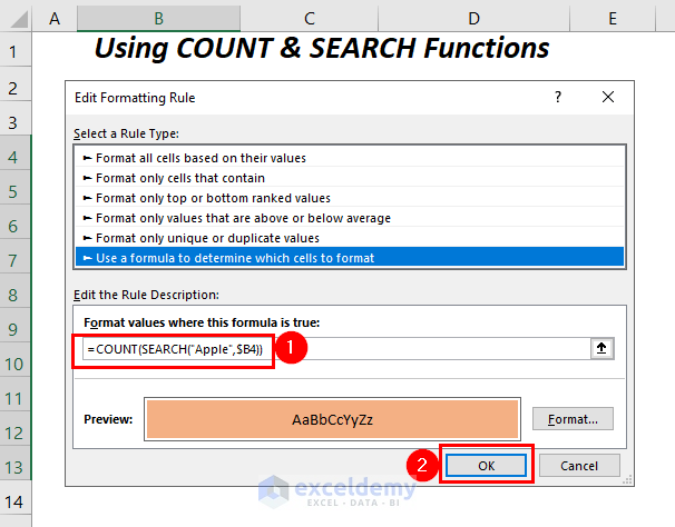
➤ Add the following formula in the Format values where this formula is true box
=COUNT(SEARCH("Apple",$B4))SEARCH will look for the portion Apple in the cells of Column B and for finding any matches it will return a value which will be the starting position of the Apple in the full text. Then, COUNT will return 1 if it gets any number from the output of the SEARCH function otherwise 0.
➤ Press OK.
Conditional Formatting will be applied to the cells of the Item column that have a part Apple or apple of the whole text.

Method-7: Using Combination of IF and SEARCH Functions
Steps:
➤ Follow Step 1 of Method 2.
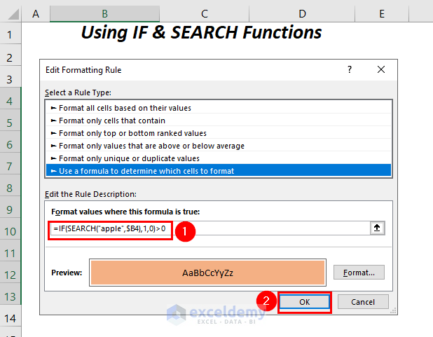
➤ Add the following formula in the Format values where this formula is true box
=IF(SEARCH("apple",$B4),1,0)>0SEARCH will look for the portion apple in the cells of Column B and for finding any matches it will return a value which will be the starting position of the apple in the full text. And then, IF will return 1 if SEARCH finds any matches otherwise 0 and for values greater than 0 finally, we will get TRUE otherwise FALSE.
➤ Press OK.
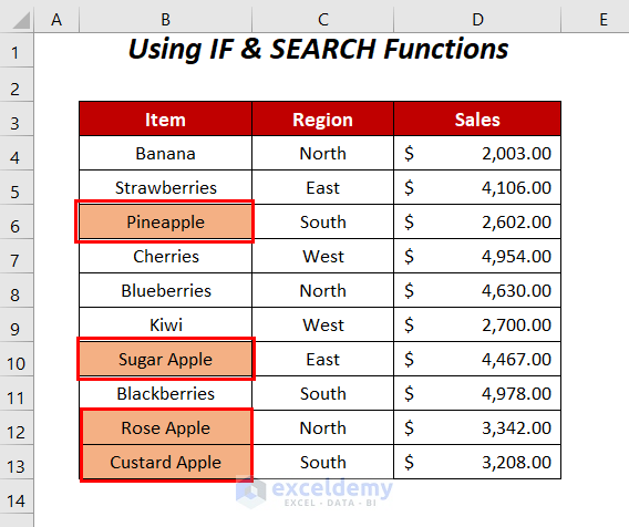
The cells having a partial match with Apple or apple will be highlighted.
Method 8 – Conditional Formatting for Partial Text Match Using MATCH Function
Steps:
➤ Follow Step 1 of Method 2.
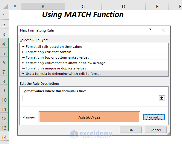
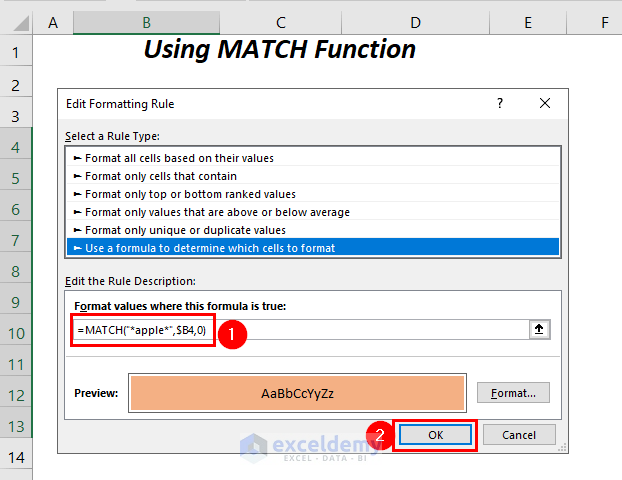
➤ Add the following formula in the Format values where this formula is true box
=MATCH("*apple*",$B4,0)By using the wildcard symbol * before and after apple we are ensuring the partial matches here and MATCH will return 1 for finding any partial matches in Column B.
➤ Press OK.
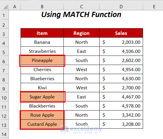
Conditional Formatting will be applied to the cells having a portion of Apple or apple in the Item column.
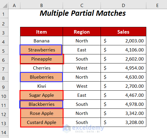
Method 9 – Conditional Formatting for Multiple Partial Text Match Using Combined Formula
Steps:
➤ Follow Step 1 of Method 2.
➤ Add the following formula in the Format values where this formula is true box
=IF(OR(ISNUMBER(SEARCH("apple", $B4)), ISNUMBER(SEARCH("berries", $B4))), "Yes", "")="Yes"- SEARCH(“apple”, $B4) → SEARCH will look for the portion apple in cell B4, and for finding any matches it will return a value which will be the starting position of the apple in the full text otherwise #N/A.
Output → #N/A
- ISNUMBER(SEARCH(“apple”, $B4)) becomes
ISNUMBER(#N/A) → ISNUMBER will return TRUE for any numeric value otherwise FALSE.
Output → FALSE
- SEARCH(“berries”, $B4) → SEARCH will look for the portion berries in cell B4, and for finding any matches it will return a value which will be the starting position of the berries in the full text otherwise #N/A.
Output → #N/A
- ISNUMBER(SEARCH(“berries”, $B4)) becomes
ISNUMBER(#N/A) → ISNUMBER will return TRUE for any numeric value otherwise FALSE.
Output → FALSE
- OR(ISNUMBER(SEARCH(“apple”, $B4)), ISNUMBER(SEARCH(“berries”, $B4))) becomes
OR(FALSE, FALSE) → OR will return TRUE if any of the values are TRUE otherwise FALSE.
Output → FALSE
- IF(OR(ISNUMBER(SEARCH(“apple”, $B4)), ISNUMBER(SEARCH(“berries”, $B4))), “Yes”, “”) becomes
IF(FALSE, “Yes”, “”) → IF will return yes for TRUE and a blank for FALSE.
Output Blank
- IF(OR(ISNUMBER(SEARCH(“apple”, $B4)), ISNUMBER(SEARCH(“berries”, $B4))), “Yes”, “”)=”Yes” becomes
“”=”Yes” → returns TRUE for matching the two values otherwise FALSE.
Output → FALSE
➤ Press OK.
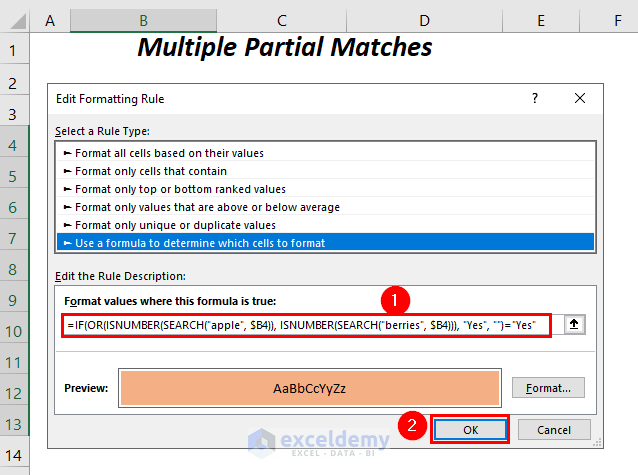
The cells with partial matches with either apple or berries will be highlighted.
Download Workbook
<< Go Back to Partial Match Excel | Formula List | Learn Excel
Get FREE Advanced Excel Exercises with Solutions!
