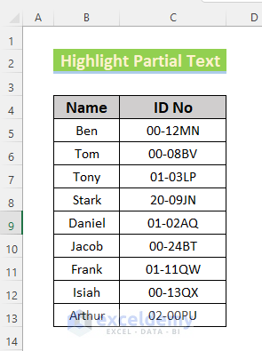
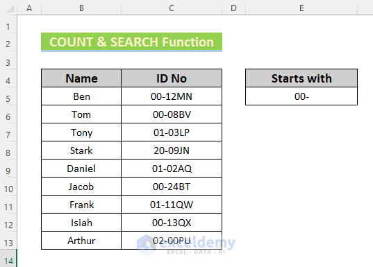
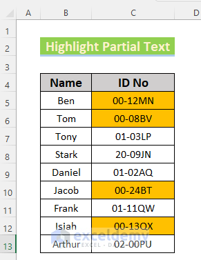
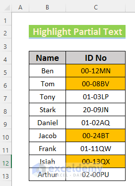
Suppose you have the following dataset.
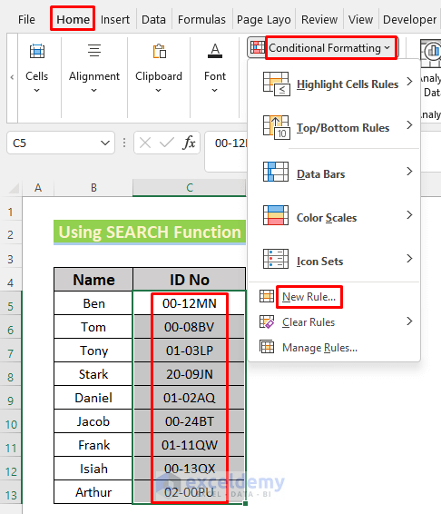
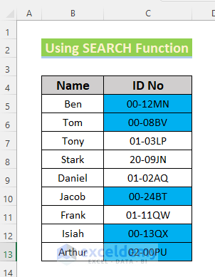
Method 1 – Using the SEARCH Function to Highlight Partial Text in Excel Cell
Steps:
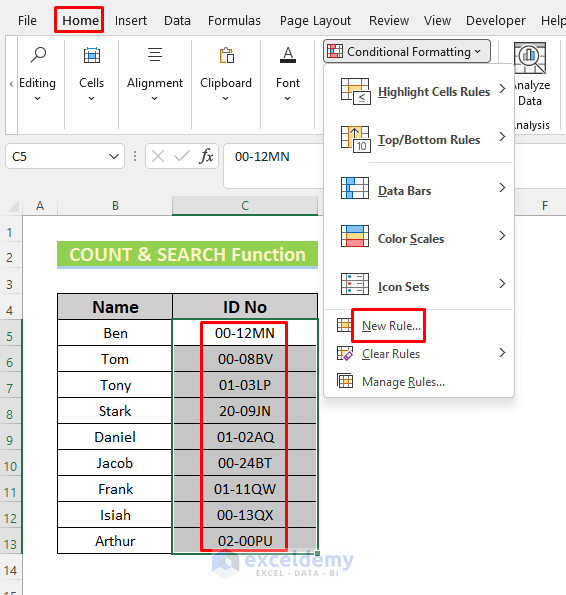
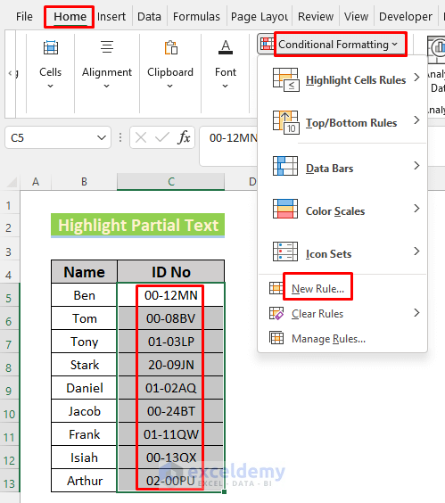
- Select the applicable range (C5:C13 in this example).
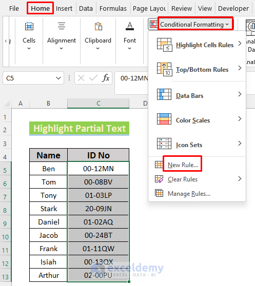
- Go to the Home ribbon and the Conditional Formatting drop-down.
- Click New Rule.
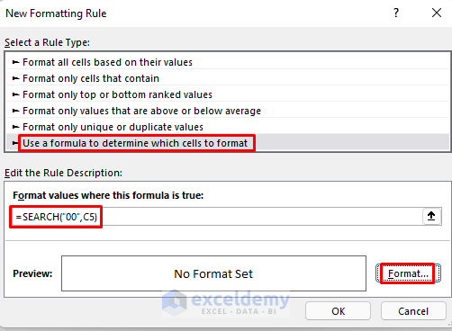
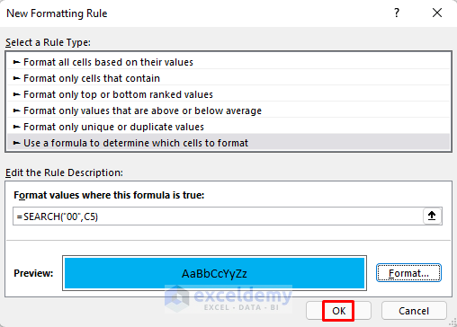
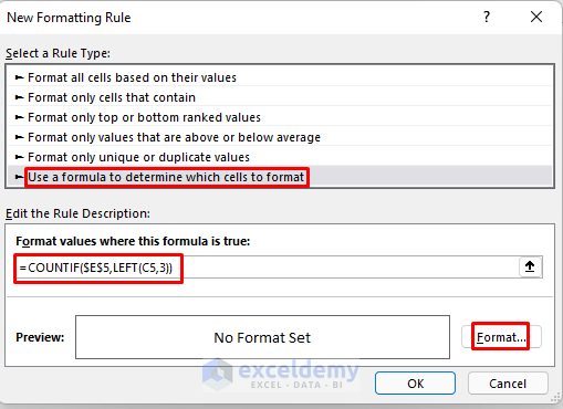
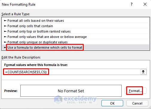
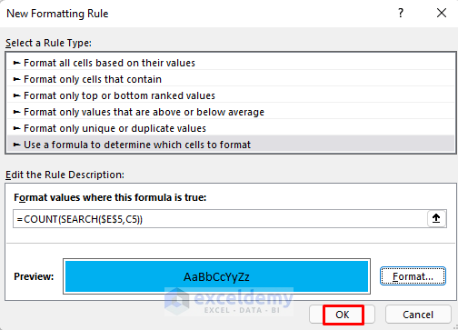
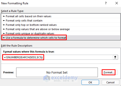
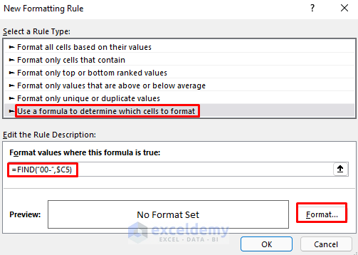
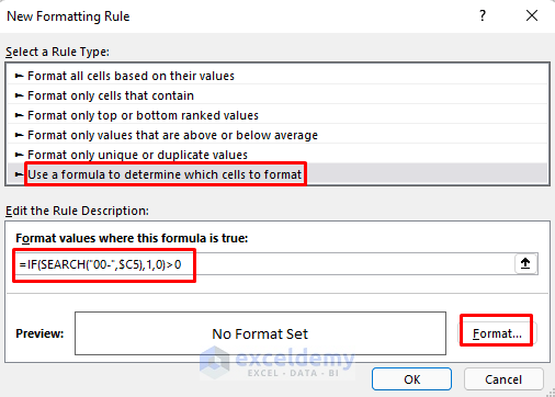
- The New Formatting Rule window will appear.
- Choose Use a formula to determine which cells to format.
- Type the following formula in Format values where this formula is true.
=SEARCH(“00”,C5)- Click Format.
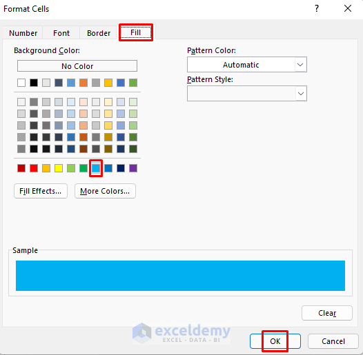
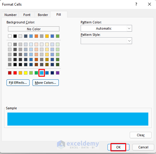
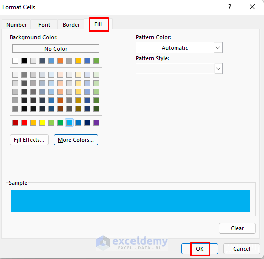
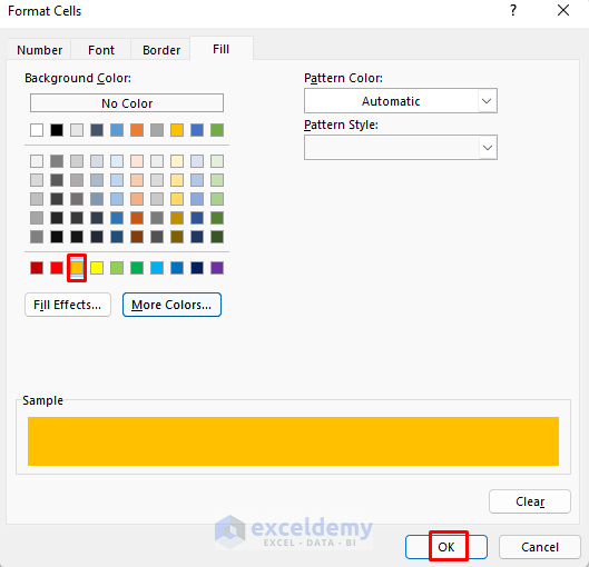
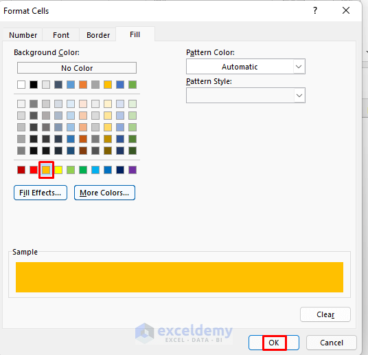
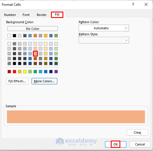
- Set the correct formatting (Number, Font, Border, Fill) for the selected cells.
- Click OK.
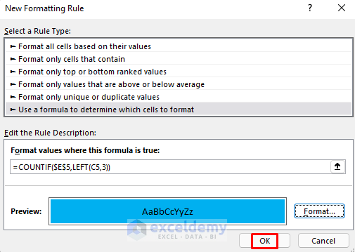
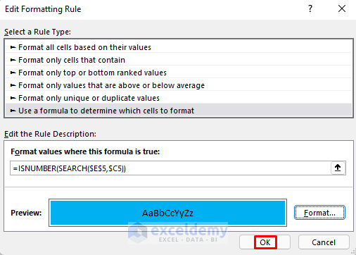
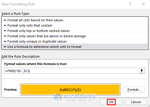
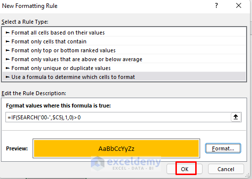
- Make sure the preview is correct.
- Click OK.
Cells with the appropriate results should now be properly formatted.
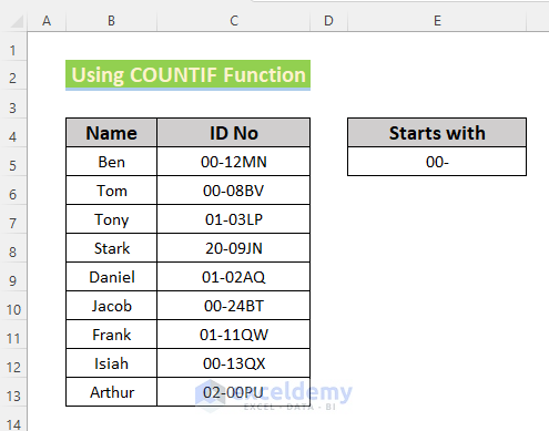
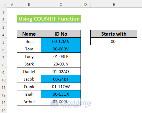
Method 2 – Applying the COUNTIF Function to Highlight Partial Text
Steps:
- Enter your criteria in a blank cell (‘00-’ in this example).
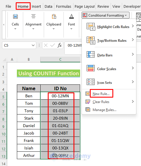
- Select the applicable range (C5:C13 in this example).
- Go to the Home ribbon and the Conditional Formatting drop-down.
- Click New Rule.
- The New Formatting Rule window will appear.
- Choose Use a formula to determine which cells to format.
- Type the following formula in Format values where this formula is true.
=COUNTIF(“00”,LEFT(C5,3))- Click on Format.
- Set the correct formatting (Number, Font, Border, Fill) for the selected cells.
- Click OK.
- Make sure the preview is correct.
- Click OK.
Cells with the appropriate results should now be properly formatted.
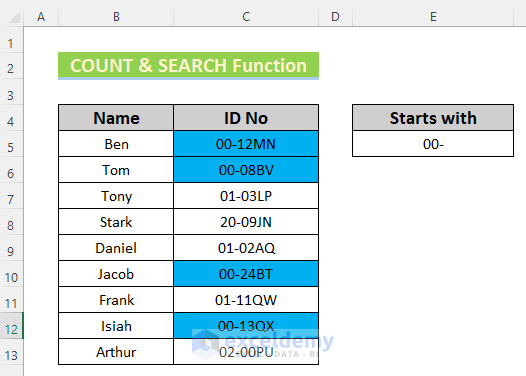
Method 3 – Utilizing the COUNT and SEARCH Functions to Highlight Partial Text
Steps:
- Enter your criteria in a blank cell (‘00-’ in this example).
- Select the applicable range (C5:C13 in this example).
- Go to the Home ribbon and the Conditional Formatting drop-down.
- Click New Rule.
- The New Formatting Rule window will appear.
- Choose Use a formula to determine which cells to format.
- Type the following formula in Format values where this formula is true.
=COUNT(SEARCH($E$5,C5))- Click on Format.
- Set the correct formatting (Number, Font, Border, Fill) for the selected cells.
- Click OK.
- Make sure the preview is correct.
- Click OK.
Cells with the appropriate results should now be properly formatted.
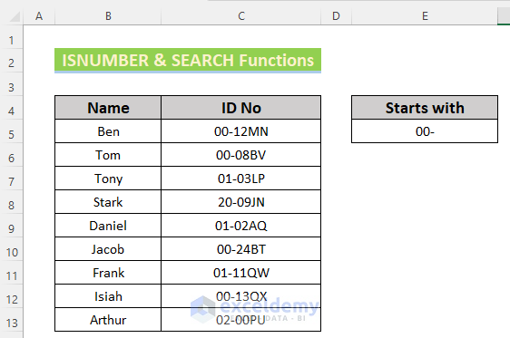
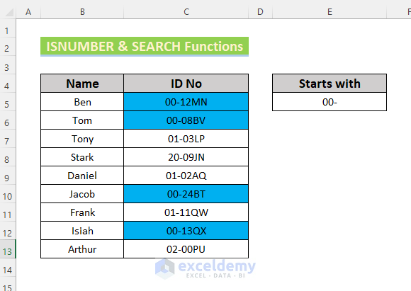
Method 4 – Using the ISNUMBER and SEARCH Functions to Highlight Partial Text
Steps:
- Enter your criteria in a blank cell (‘00-’ in this example).
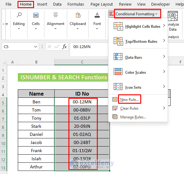
- Select the applicable range (C5:C13 in this example).
- Go to the Home ribbon and the Conditional Formatting drop-down.
- Click New Rule.
- The New Formatting Rule window will appear.
- Choose Use a formula to determine which cells to format.
- Type the following formula in Format values where this formula is true.
=ISNUMBER(SEARCH($E$5,$C5))- Click on Format.
- Set the correct formatting (Number, Font, Border, Fill) for the selected cells.
- Click OK.

- Make sure the preview is correct.
- Click OK.
Cells with the appropriate results should now be properly formatted.
Method 5 – Utilizing the FIND Function to Highlight Partial Text
Steps:
- Select the applicable range (C5:C13 in this example).
- Go to the Home ribbon and the Conditional Formatting drop-down.
- Click New Rule.
- The New Formatting Rule window will appear.
- Choose Use a formula to determine which cells to format.
- Type the following formula in Format values where this formula is true.
=FIND("00-",$C5)- Click on Format.
- Set the correct formatting (Number, Font, Border, Fill) for the selected cells.
- Click OK.
- Make sure the preview is correct.
- Click OK.
Cells with the appropriate results should now be properly formatted.
Method 6 – Combining IF and SEARCH Functions
Steps:
- Select the applicable range (C5:C13 in this example).
- Go to the Home ribbon and the Conditional Formatting drop-down.
- Click New Rule.
- The New Formatting Rule window will appear.
- Choose Use a formula to determine which cells to format.
- Type the following formula in Format values where this formula is true.
=IF(SEARCH("00-",$C5),1,0)>0- Click on Format.
- Set the correct formatting (Number, Font, Border, Fill) for the selected cells.
- Click OK.
- Make sure the preview is correct.
- Click OK.
Cells with the appropriate results should now be properly formatted.
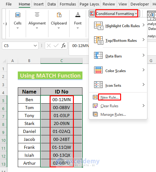
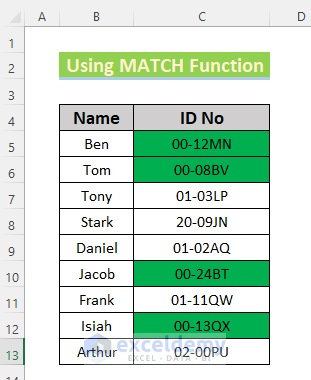
Method 7 – Applying the MATCH Function to Highlight Partial Text
Steps:
- Select the applicable range (C5:C13 in this example).
- Go to the Home ribbon and the Conditional Formatting drop-down.
- Click New Rule.
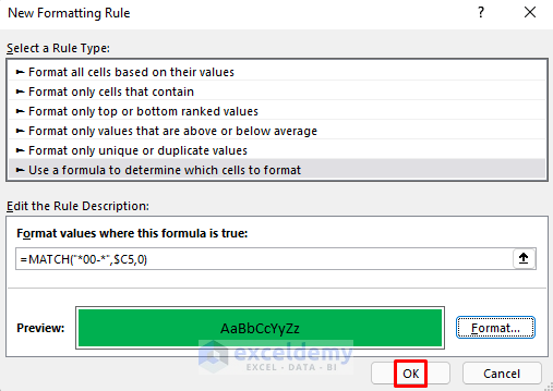
- The New Formatting Rule window will appear.
- Choose Use a formula to determine which cells to format.
- Type the following formula in Format values where this formula is true.
=MATCH("*00-*",$C5,0)- Click on Format.
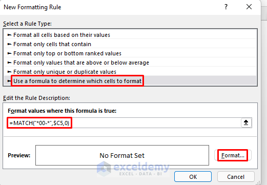
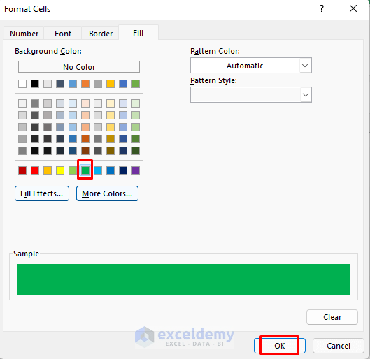
- Set the correct formatting (Number, Font, Border, Fill) for the selected cells.
- Click OK.
- Make sure the preview is correct.
- Click OK.
Cells with the appropriate results should now be properly formatted.
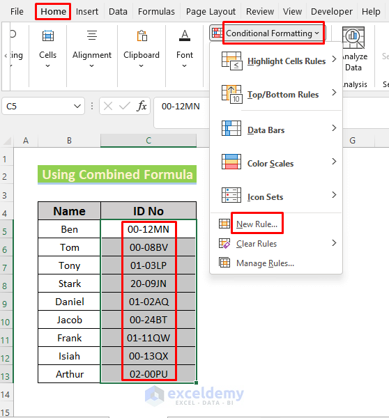
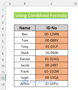
Method 8 – Use of the Combined Formula
Steps:
- Select the applicable range (C5:C13 in this example).
- Go to the Home ribbon and the Conditional Formatting drop-down.
- Click New Rule.
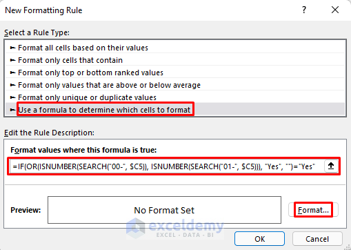
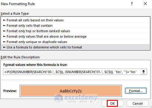
- The New Formatting Rule window will appear.
- Choose Use a formula to determine which cells to format.
- Type the following formula in Format values where this formula is true.
=IF(OR(ISNUMBER(SEARCH("00-", $C5)), ISNUMBER(SEARCH("01-", $C5))), "Yes", "")="Yes"- Click on Format.
Formula Breakdown (using this example)
SEARCH(“00-”, $C5) → The SEARCH function will return the position of the text ‘00-’ from the ID No in cell C5 if it finds a match otherwise it will return #N/A (Value not Available Error).
Output: 1
ISNUMBER(SEARCH(“00-”, $C5)) becomes
ISNUMBER(1) → ISNUMBER returns TRUE for any numeric value, else, it returns FALSE.
Output: TRUE
SEARCH(“01-”, $C5) → Turns into
Output: #N/A
ISNUMBER(SEARCH(“01-”, $C5)) → becomes
ISNUMBER(#N/A) → returns
Output: FALSE
OR(ISNUMBER(SEARCH(“00-”, $C5)), ISNUMBER(SEARCH(“01-”, $C5))) → Turns into
OR(TRUE, FALSE) → OR function returns TRUE if any of the values are TRUE otherwise it results in FALSE.
Output: TRUE
IF(OR(ISNUMBER(SEARCH(“00-”, $C5)), ISNUMBER(SEARCH(“01-”, $C5))), “Yes”, “”) → becomes
IF(TRUE, “Yes”, “”) → IF will return yes for TRUE and a blank for FALSE.
Output: Yes
IF(OR(ISNUMBER(SEARCH(“00-”, $C5)), ISNUMBER(SEARCH(“01-”, $C5))), “Yes”, “”)=”Yes” → turns into
“Yes”=”Yes” → returns TRUE the two values match with each other but on the contrary, it returns FALSE.
Output: TRUE
- Set the correct formatting (Number, Font, Border, Fill) for the selected cells.
- Click OK.
- Make sure the preview is correct.
- Click OK.
Cells with the appropriate results should now be properly formatted.
Method 9 – Application of VBA
Steps:
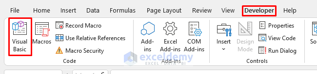
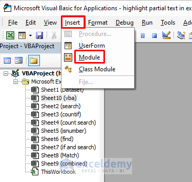
- Open Visual Basic from the Developer Tab.
- The VBA window will open. Select Insert then Module.
- Type the following code in the VBA Module.
Sub Highlight_Partial_Text()
Dim row_number As Integer, col_number As Integer
Dim Partial_Text_Cell As String
col_number = 2
For row_number = 5 To 13
    Partial_Text_Cell = ActiveSheet.Cells(row_number, col_number).Value
    TextPosition1 = InStr(1, Partial_Text_Cell, "Ben")
    TextPosition2 = InStr(1, Partial_Text_Cell, "Frank")
    If TextPosition1 > 0 Then
        ActiveSheet.Cells(row_number, col_number).Characters(TextPosition1, 3).Font.Color = RGB(255,0,0)
    End If
    If TextPosition2 > 0 Then
        ActiveSheet.Cells(row_number, col_number).Characters(TextPosition2, 5).Font.Color = RGB(255,0,0)
    End If
Next row_number
End Sub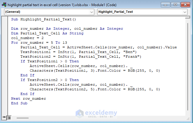
row_number and col_number are Integer variables and Partial_Text_Cell is a string variable.
The IF Statement within the For Loop will change the Text Postions’ font color by the VBA Font.Color property.
- Go back to the worksheet and run Macros.
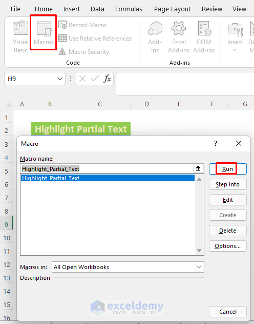
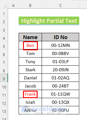
- Cells with the appropriate results should now be properly formatted.
Download Practice Workbook
<< Go Back to Partial Match Excel | Formula List | Learn Excel
Get FREE Advanced Excel Exercises with Solutions!
