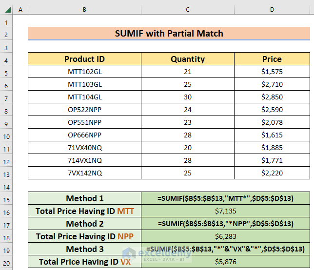
In this tutorial, we will describe how to use the SUMIF function based on a partial match in three different scenarios: at the beginning of a value, at the end, and at any position within the value respectively.
Here is a quick summary of what we’ll cover:
Overview of the SUMIF Function
The SUMIF function is used to sum values that meet a specific criterion. For example, if we want to add up all the values in a column that are greater than 20, we would specify that as the condition in the SUMIF function.
Syntax:
Arguments:
- range: The range of cells to be added together (required).
- criteria: The condition based on which to perform the sum operation within the range (required). The conditions can be specified as follows: 20, “>20”, F2, “15?”, “Car*”, “*~?”, or TODAY().
- sum_range: The cell range to include in the sum formula, excluding the range argument (optional).
How to Use the SUMIF Function for a Partial Match in Excel: 3 Ways
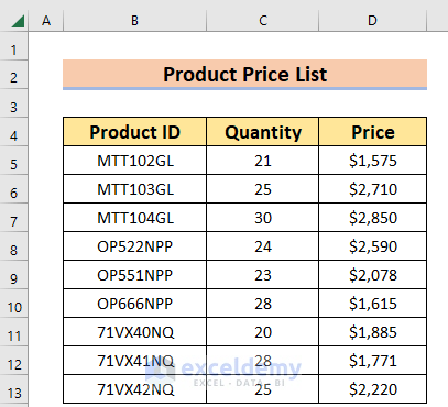
We’ll use the following Product Price List data table to demonstrate our methods.
Method 1 – Using SUMIF for a Partial Match at the Beginning
In our first example, we’ll sum only if we find a match at the beginning of a cell value. For example, let’s add up the values of only those products from the Product Price List table whose Product ID starts with “MTT”.
Steps:
- Select cell C16 to store the formula result.
- Enter the following formula in cell C16:
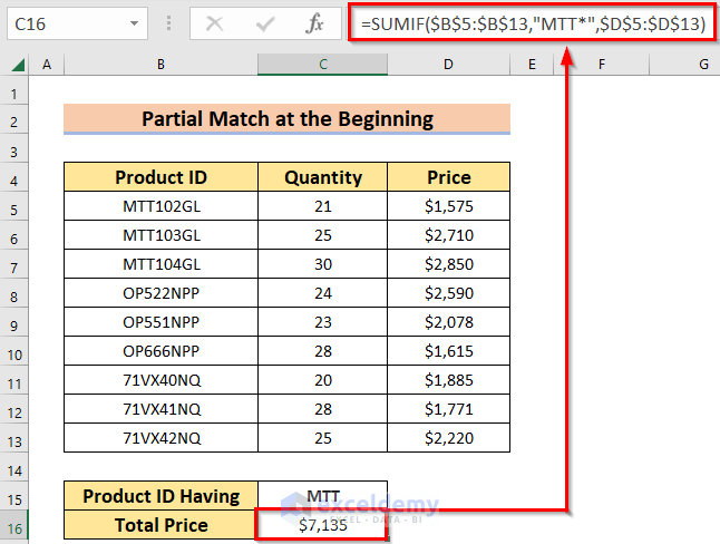
=SUMIF($B$5:$B$13,"MTT*",$D$5:$D$13)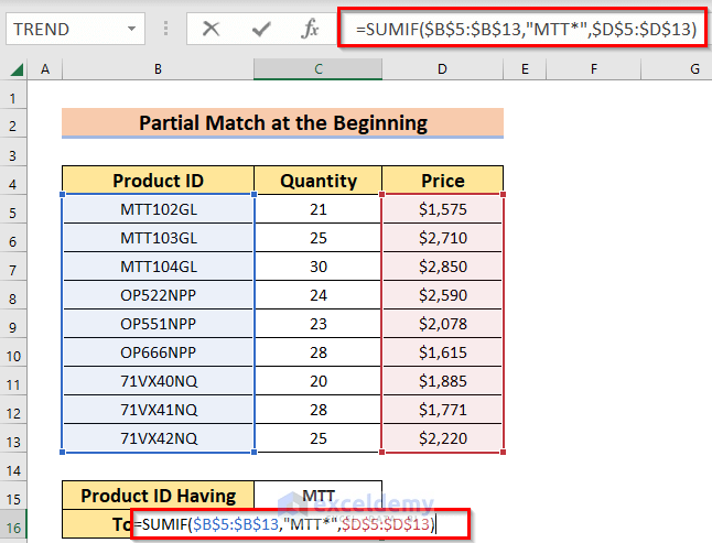
- Press ENTER.
Formula Breakdown:
- $B$5:$B$13 : refers to the cell range of the Product ID column. Within this range, we will look for the keyword “MTT”.
- “MTT*” : the keyword to search that must appear at the beginning of the product IDs.
- $D$5:$D$13 : the sum range where the summing operation will be executed.
=SUMIF($B$5:$B$13,"MTT*",$D$5:$D$13) : returns the sum of the prices for only those products having the “MTT” keyword at the beginning of their Product IDs.- Output: $7,135.
Method 2 – Using SUMIF for a Partial Match at the End
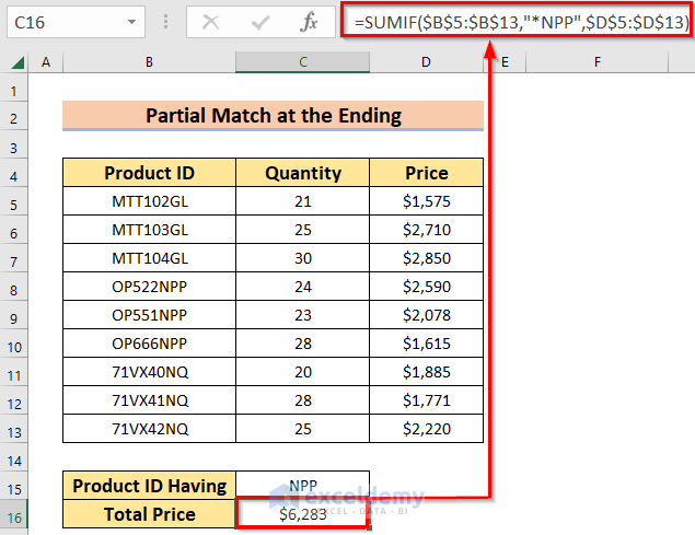
Now, we will calculate the sum of the prices of only the products that have the keyword “NPP” at the end of their Product IDs.
Steps:
- Select cell C16 to store the formula result.
- Enter the following formula:
=SUMIF($B$5:$B$13,"*NPP",$D$5:$D$13)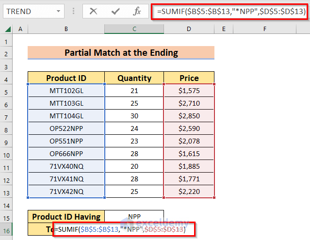
- Press ENTER.
Formula Breakdown:
- $B$5:$B$13 : the cell range of the Product ID column, where we will look for the keyword “NPP”.
- “*NPP” : the keyword to search that must appear at the end of the product IDs.
- $D$5:$D$13 : the sum range where the summing operation will be executed.
=SUMIF($B$5:$B$13,"*NPP",$D$5:$D$13): returns the sum of the prices of only those products having the “NPP” keyword at the end of their Product IDs.- Output: $6,283.
Method 3 – Using SUMIF for a Partial Match at Any Position
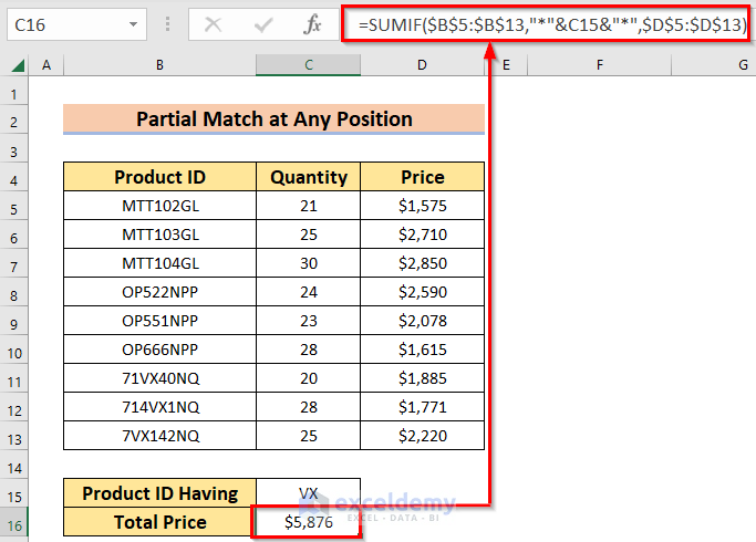
In this last example, we’ll present a universal formula that can perform the sum operation based on a partial match at any position in a cell value. For example, let’s add the prices of only those products containing the keyword “VX” in any position in their Product ID.
Steps:
Select cell C16 to store the formula result.
Enter the following formula in the cell:
=SUMIF($B$5:$B$13,"*"&C15&"*",$D$5:$D$13)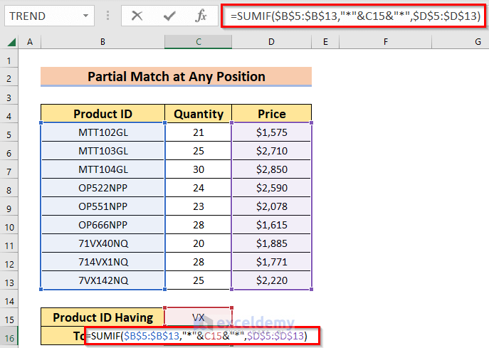
Press ENTER.
Formula Breakdown:
- $B$5:$B$13 : the cell range of the Product ID column, where we will look for the keyword “VX”.
- “*”&C15&”*” : the cell address C15 holds the search keyword “VX”. You can use cell C15 as a search box, where you can input any keyword to search for and then sum the corresponding prices of matched values in the range.
- $D$5:$D$13 : the sum range where the summing operation will be executed.
=SUMIF($B$5:$B$13,"*"&C15&"*",$D$5:$D$13): returns the sum of the prices of only those products having the “VX” keyword in any position within their Product IDs.- Output: $5,876.
Things to Remember
- Be careful with the positioning of the asterisk (*) in the criteria field.
- Make sure the range you are selecting for the range and sum_range arguments are correct.
Download Practice Workbook
<< Go Back to Partial Match Excel | Formula List | Learn Excel
Get FREE Advanced Excel Exercises with Solutions!
