Method 1 – Using VLOOKUP with Wildcard for Partial/Exact Match from a Column
Steps:
- Enter the following formula in cell C15 and press the Enter key.
=VLOOKUP("*"&C14&"*",B5:E12,1,FALSE)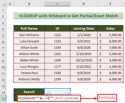
Formula Breakdown:
- In the first argument, “*”&C14&”*” is the lookup value. We are using wildcard characters to check the lookup value.
- B5:E12 this is the range where we will search the value.
- 1 is used to extract the data from the first column.
- FALSE is used to define the exact match.
- Enter any keyword in cell C14 and press the Enter key.
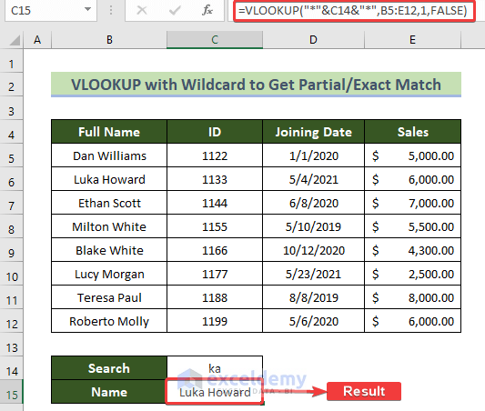
Find a partial match for any number of characters and within any part of the text from the lookup range by using the VLOOKUP function with wildcards.
Method 2 – Achieving Partial Matched Data from a Range with VLOOKUP Function
Steps:
- Click on cell C16 and insert the following formula.
=VLOOKUP("*"&C14&"*",B5:E12,3,FALSE)The main difference is that we want to extract the Joining Date from the 3rd column, that’s why 3 is given as the column index.
- Press the Enter key.
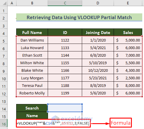
- Enter any keyword in the search box on cell C14 and press Enter.
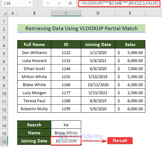
TRetrieve multiple-column data with the VLOOKUP function by partial match.
Method 3 – Getting Partial Match of Numerical Data with Excel VLOOKUP Function
Steps:
- Click on cell C17 and insert the following formula.
=VLOOKUP("*"&C14&"*",B5:E12,4,FALSE)- Press the Enter key.
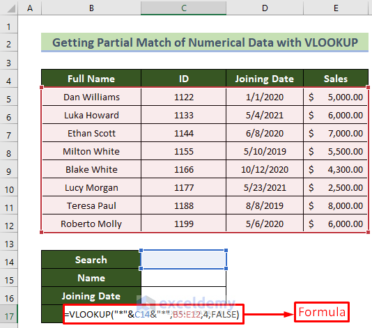
Formula Breakdown:
- To extract Salary from the 3rd column, 4 is the column index.
- Enter any keyword in the search box on cell C14 and press the Enter key.
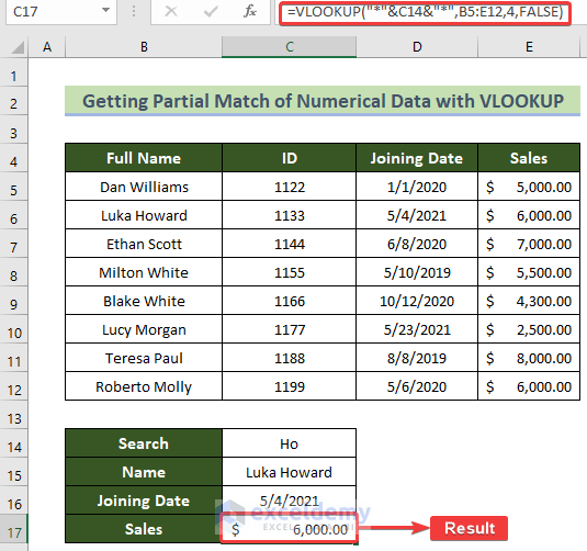
You will be able to lookup for multiple values with partial matches including numerical values.
Method 4 – Searching Data with VLOOKUP for Partial Match and Conditions
- Enter the following formula in cell C16 and press the Enter key.
=IF(VLOOKUP(C15,B5:E12,4)>=E15,"Yes","No")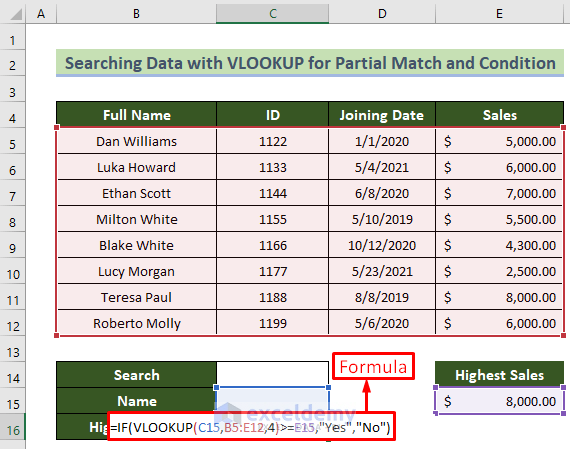
Formula Breakdown:
- VLOOKUP(C15, B5:E12,4)>=E15 is the logical condition of the IF function here. We are checking whether the entered name has the highest sales or not.
- If the entered name’s salary matches our already defined highest salary, it will return “Yes,” otherwise “No.”
- To learn more about the IF function, you can check this link.
- Enter any keyword in the search box on cell C14 and press the Enter key.
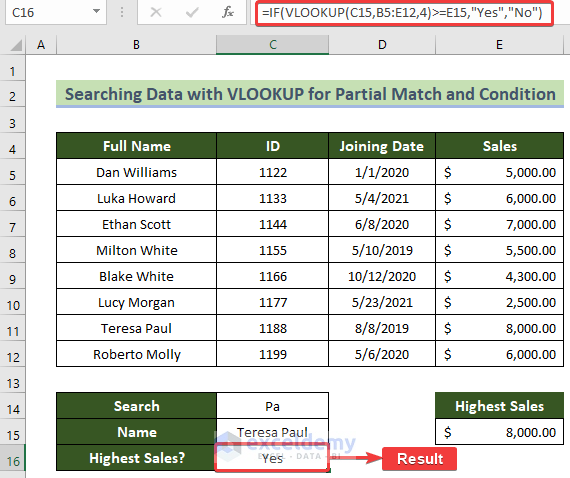
Find the conditional answer in cell C16 with a partial match for the VLOOKUP function.
Excel VLOOKUP Not Working for Partial Match: What Are the Reasons?
The VLOOKUP function with partial match is an intricate task sometimes. So, you might find errors or fail to get the desired result for several reasons. The main reasons for the VLOOKUP partial match not working are given as follows.
- If the wild card character is in the wrong placement.
- If the column number is inappropriate inside the VLOOKUP function.
- If the search value does not exist in the source data’s lookup region, you will get the #N/A errors.
- If there is extra space or unnecessary characters inside the search value or source range values.
- If there are multiple matches for a single lookup value, then the first lookup value will be shown in the result.
INDEX-MATCH: An Alternative to VLOOKUP for Partial Match in Excel
Steps:
- Enter the following formula in cell C15 and press the Enter key.
=INDEX($B$5:$B$12,MATCH("*"&C14&"*",$B$5:$B$12,0))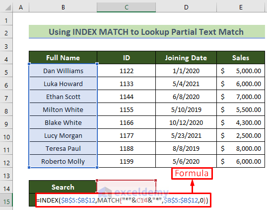
Formula Breakdown:
- See the inner function which is MATCH. The first argument “*”&C14&”*” this matches the data with our partial text in the Model column. $B$5:$B$12 this is the Model column range. 0 is used to define the exact match.
- Afterward, in the INDEX function, $B$5:$B$12 is the range where we will find the index. The MATCH data’s return result will be considered a row number.
- Enter any keyword in the search box on cell C14 and press the Enter key.
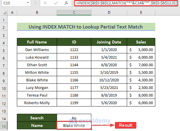
You will get your desired result in cell C15 using the INDEX-MATCH combination.
VLOOKUP Partial Match: Knowledge Hub
- How to Use VLOOKUP to Find Partial Text from a Single Cell
- How to Vlookup Partial Match for First 5 Characters in Excel
- Excel VLOOKUP for Partial Match in Table Array
- How to Use Excel VLOOKUP to Find the Closest Match
- How to Use VLOOKUP to Find Approximate Match for Text in Excel
<< Go Back to Excel VLOOKUP Function | Excel Functions | Learn Excel
Get FREE Advanced Excel Exercises with Solutions!
