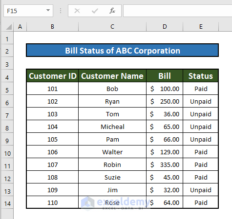
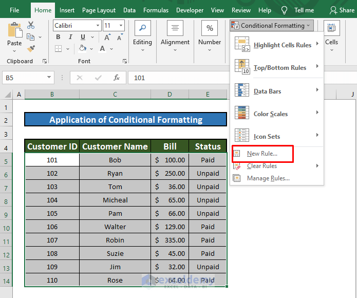
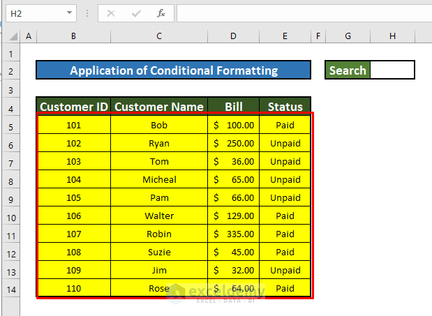
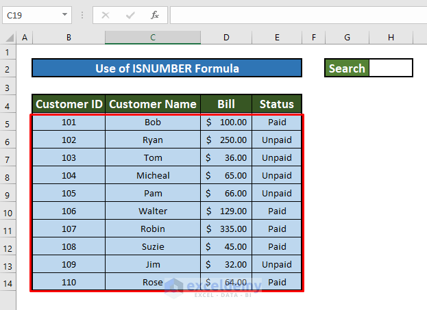
We have a dataset regarding the Bill Status of a Corporation. This dataset consists of four columns: Customer ID, Customer Name, Bill, and Status. We have 10 rows of data in the worksheet. We will create a search box to go through the dataset.
Method 1 – Use Conditional Formatting to Create a Search Box in Excel
Steps:
- Make a cell where you want to search for any data. We have selected the H2 cell.
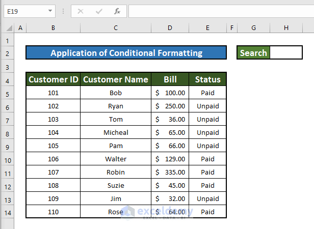
- Select the range B5:E14.
- Go to the Home tab on the toolbar and select Conditional Formatting.
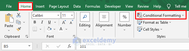
- Under Conditional Formatting, click on the New Rule option.
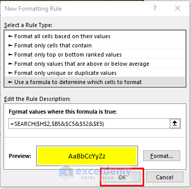
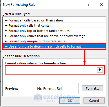
- You’ll get a New Formatting Rule window. Select the option Use a formula to determine which cells to format.
- You’ll get a Formula Bar.
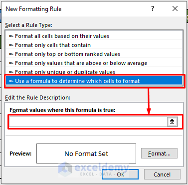
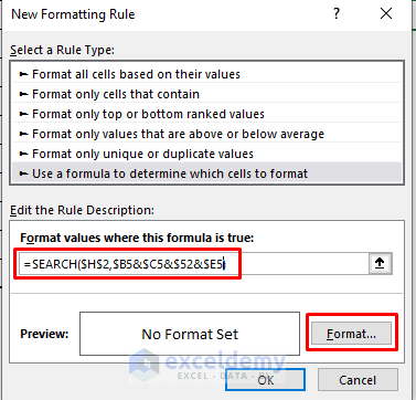
- Enter the formula given below in the box.
=SEARCH($H$2,$B5&$C5&$D5&$E5)- Go to Format.
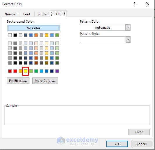
- Select a color to see the searched result in the dataset from the Fill tab. We have selected a yellow color.
- Press the OK button.
- You’ll get the preview of the formatting. Press OK.
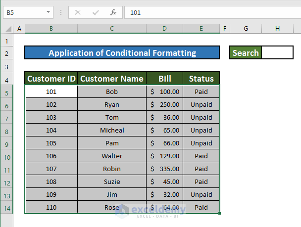
- The whole dataset will be highlighted since the search box is empty.
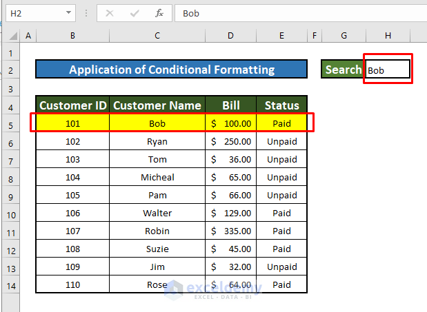
- In cell H2, enter any text, and you will find the resulting row highlighted in yellow.
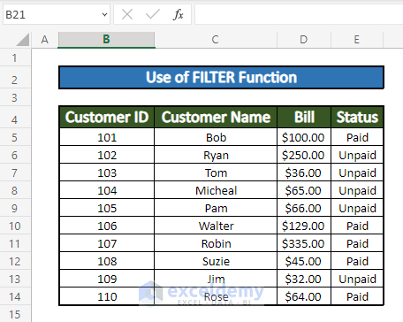
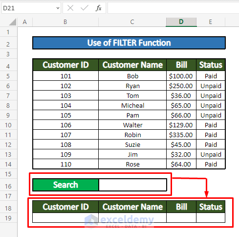
Method 2 – Use the FILTER Function to Create a Search Box in Excel
Steps:
- We’ll use the same dataset.
- Select a cell to make a search box. We’ll use cell C16. Add borders and some surrounding formatting if you want.
- Make a result box from B18 to E19. This will display the resulting rows.
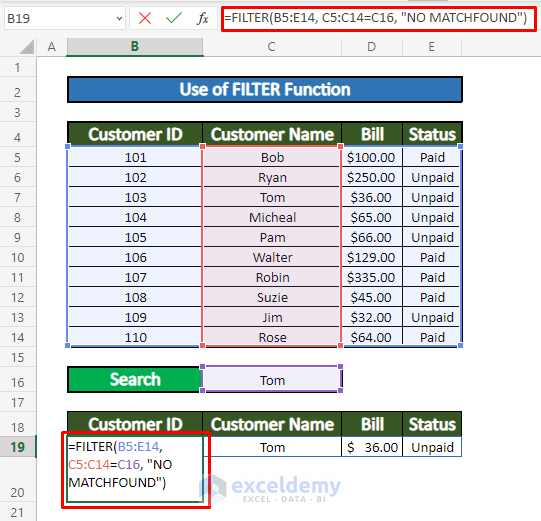
- In cell B19, enter the formula given below:
=FILTER(B5:E14,C5:C14=C16, “NO MATCH FOUND”)In this formula, B5:E14 is the range of values to be filtered, C5:C14=C16 is the criteria to be matched, and “NO MATCH FOUND” is the value to be returned when no entries meet the criteria.
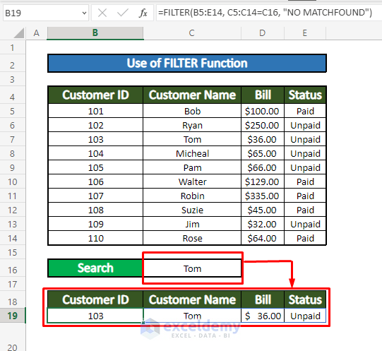
- Enter a name into the search box. You will see the whole result.
Read More: How to Create a Filtering Search Box for Your Excel Data
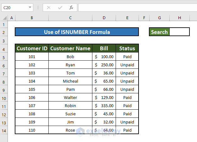
Method 3 – Create a Search Box Using the ISNUMBER Function
Steps:
- Select the H2 cell to make a search box and format it a bit (see image).
- From the ribbon, select the Home tab.
- Go to Conditional Formatting and select New Rule.
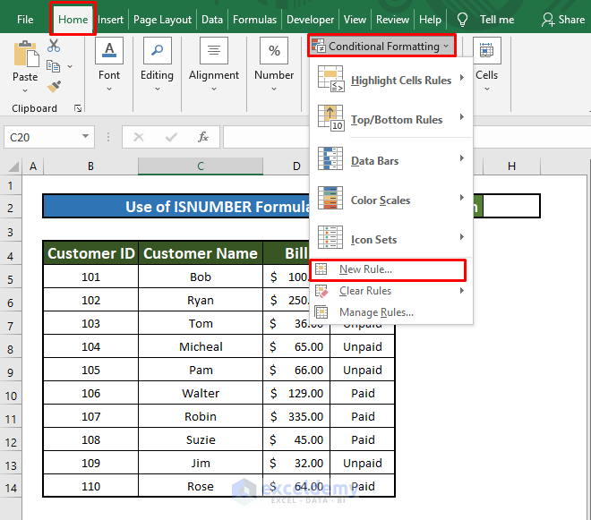
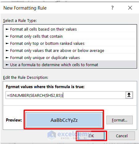
- Select the option Use a formula to determine which cells to format.
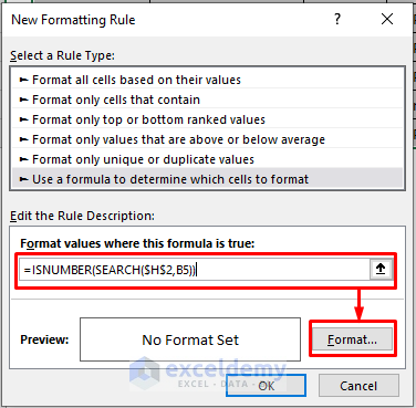
- In the formula bar, insert the formula given below:
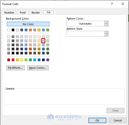
=ISNUMBER(SEARCH($H$2,B5))- Cick on the Format button.
- From the Fill tab, select any color. We have selected a blue color.
- Press OK.
- You can preview the selected color. Press OK.
- You will see the whole dataset with the same blue color after formatting.
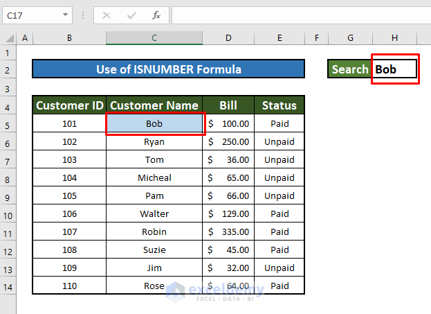
- Search for a value in the search box. You will find the result filled with blue color.
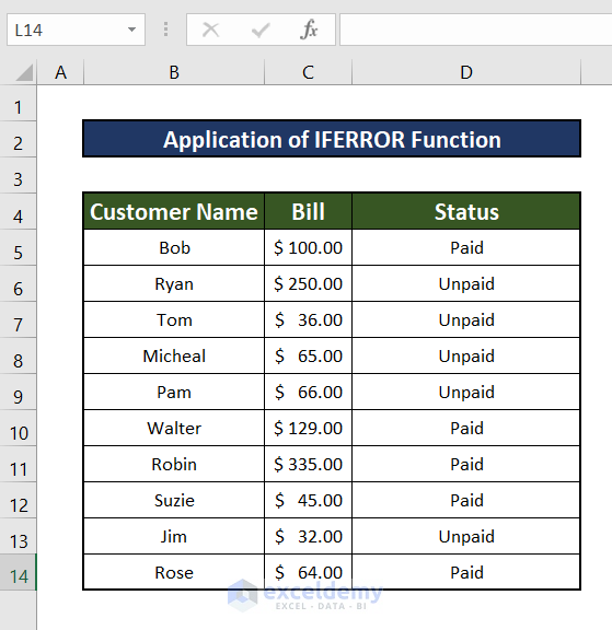
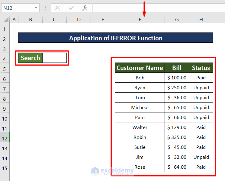
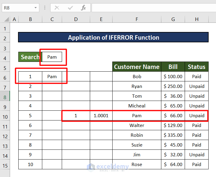
Method 4 – Apply the IFERROR Function to Create a Search Box in Excel
Steps:
- We’ll use a different dataset ranging from B4 to D14.
- We moved our dataset from B4-D14 to F5-H14.
- Select cell C4 to make a search box.
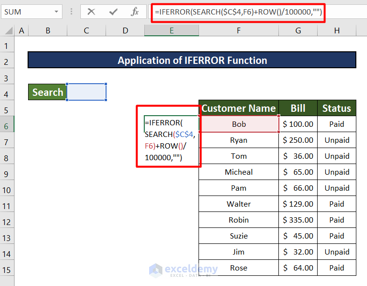
- In E6, enter the formula given below:
=IFERROR(SEARCH($C$4,F6)+ROW()/100000,"")- $C$4 is the text which is going to be searched.
- F6 is the cell number to perform the search.
- After searching, the function returns a value. This value is added to the ROW number, and then divided by 100000.
- The IFERROR function returns the exact value if there is no error.
- “” is the argument meaning the IFERROR function will return nothing if there is no error.
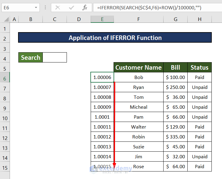
- Use the Fill Handle to paste the formula from E6 to E15.
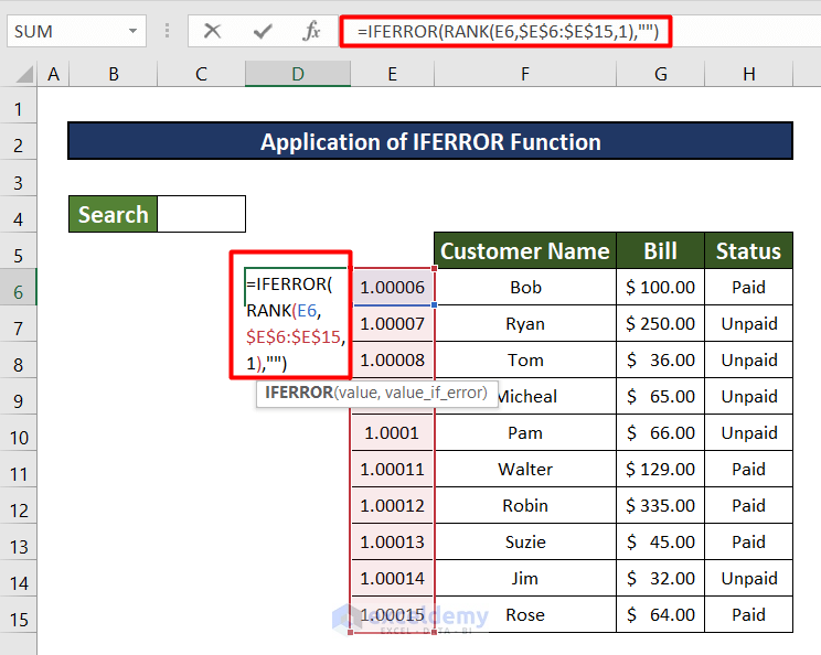
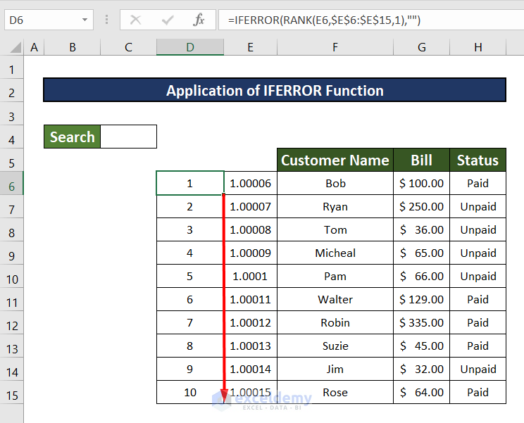
- In D6, enter the formula given below:
=IFERROR(RANK(E6,$E$6:$E$15,1),"")- E6 is a value for which we will find the rank.
- $E$6:$E$15 is a range of cells to be ranked.
- 1 is a number to specify the order. Here, 1 is for ascending order.
- The IFERROR function will work just like explained earlier.
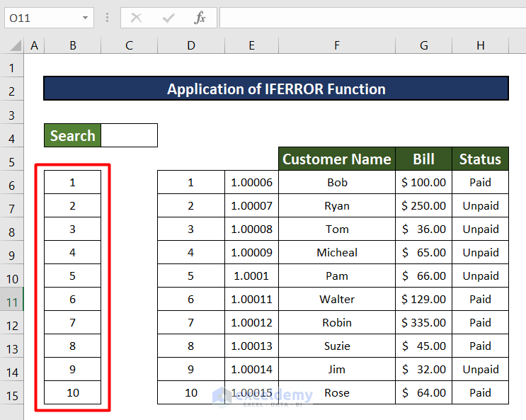
- Use the Fill Handle copy the formula from D6 to D15.
- Input numbers from B6 to B15 into D6 to D15.
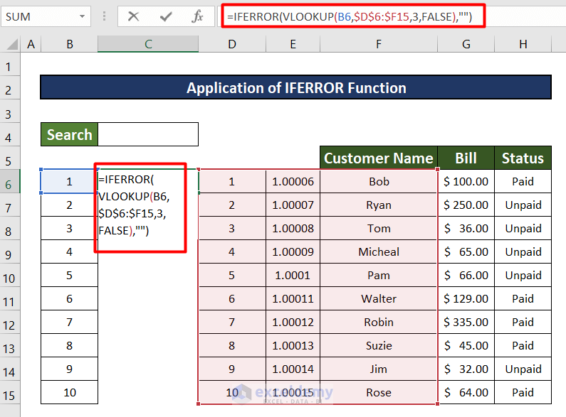
- In the C6 cell, input the formula given below:
=IFERROR(VLOOKUP(B6,$D$6:$F15,3,FALSE),"")- B6 is the cell that you want to look up.
- $D$6:$F15 is the range of cells you want to look for.
- 3 is the column number in the range to return the containing value.
- FALSE indicates to return a match.
- Then the IFERROR function will work just like explained earlier.
- Use the Fill Handle to input the formula to the whole column.
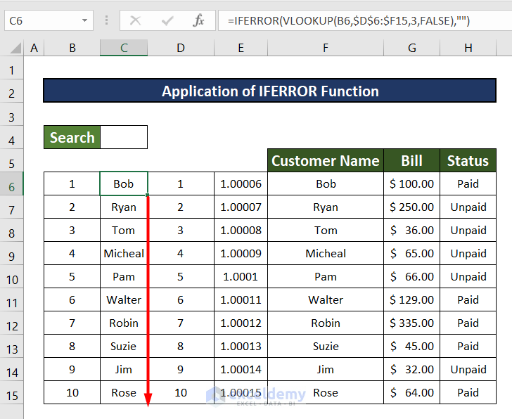
- Input data into the search box. You can see the result below.
- You can apply additional formatting or hide the helper columns.
Things to Remember
- You need to use Excel 365 for the FILTER function.
- The VLOOKUP Function only looks up from right to left.
Download the Practice Workbook
Related Articles
- Create a Search Box in Excel with VBA
- How to Create a Search Box in Excel Without VBA
- How to Create a Search Box in Excel for Multiple Sheets
<< Go Back to Data Management in Excel | Learn Excel
Get FREE Advanced Excel Exercises with Solutions!
