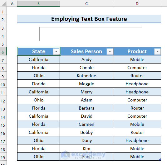
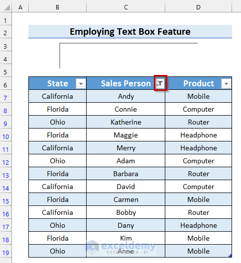
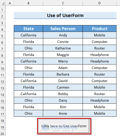
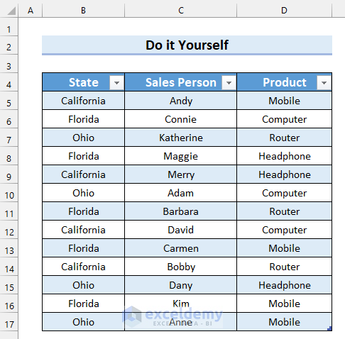
Create a Search Box in Excel with VBA (5 Suitable Examples)

We have taken the following table as the dataset. This table contains State, Sales Person, and Product columns. We will create a search box in Excel with VBA for this table.

Example 1 – Using the Text Box Feature to Create a Search Box in Excel

Steps:

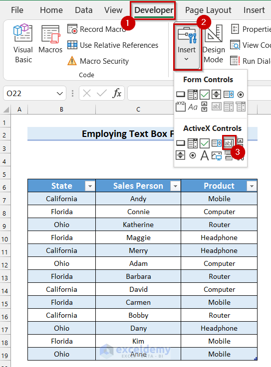
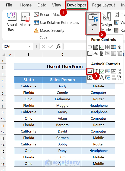
Go to the Developer tab.
Select Insert. A drop-down menu will appear.
Select Text Box from ActiveX Controls.

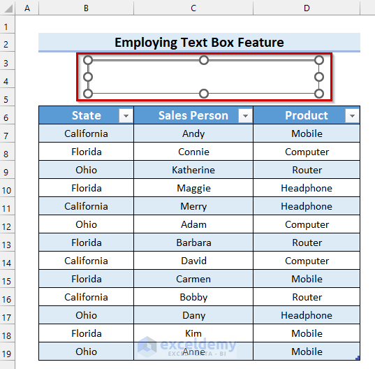
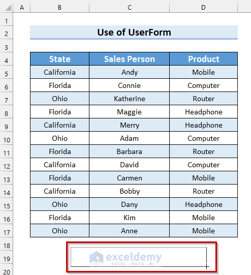
Click and drag your mouse cursor where you want your Text Box.

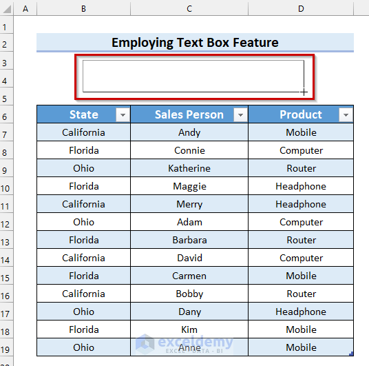
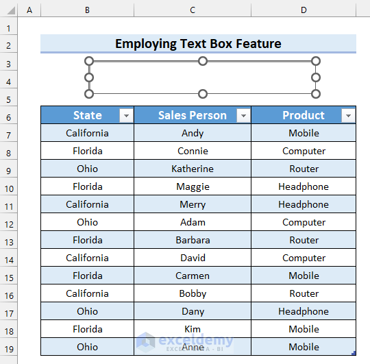
You will see a Text Box inserted into your worksheet.

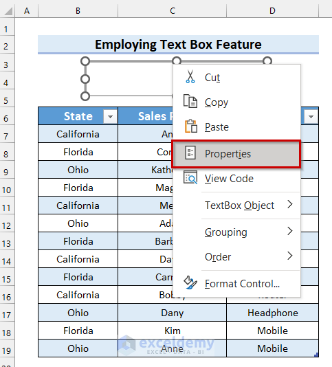
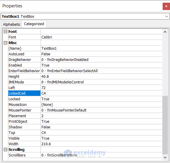
Right-click on the Text Box.
Select Properties.

Select a blank cell as a LinkedCell. We selected cell C4.

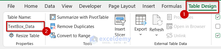
We will name the table to use the name in the VBA code.
Select any cell from the table. We selected cell B6.

Go to the Table Design tab.
Name the table as you want. We named it TextBox_Data.

Double-click on the Text Box.

A Module will open with a Private Sub on it.
Use the following code in that Module.

Private Sub TextBox1_Change()
Application.ScreenUpdating = False
ActiveSheet.ListObjects("TextBox_Data").Range.AutoFilter field:=2, Criteria1:=[c4] & "*", Operator:=xlFilterValues
Application.ScreenUpdating = True
End Sub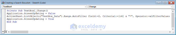

Code Breakdown

A Private Sub Procedure was already created by the Text Box. A Private Sub is only applicable for that specific sheet it is on.
We set Application.ScreenUpdating property as False to speed up the macro.
We used the ListObjects property to return the table named “TextBox_Data”.
We used Range.AutoFilter method to filter the range. We selected 2 for field which will filter the 2nd column of the table and we selected [C4] & “*” as Criteria1 which will match the 1st letter with the input in search box. For Operator, we selected xlFilterValues which will filter the values.
We set Application.ScreenUpdating property as True because we have reached the last part of the macro.

Save the code and go back to the worksheet.
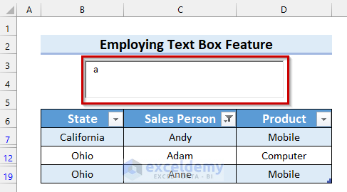
You will get a filter added to the Sales Person column.

You can search in the search box for whatever you want. We searched for “a” and the names that start with “a” have appeared.

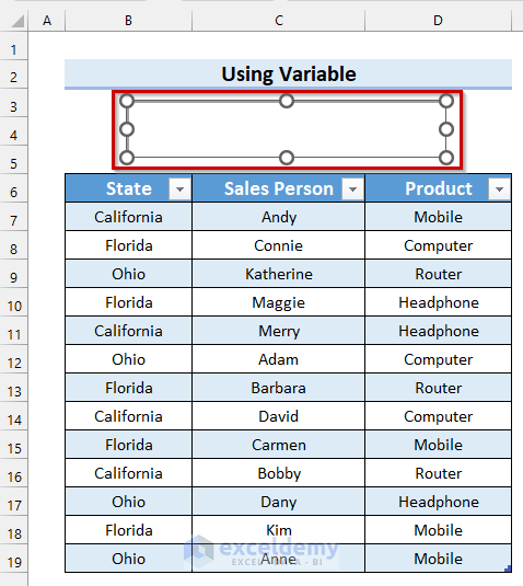
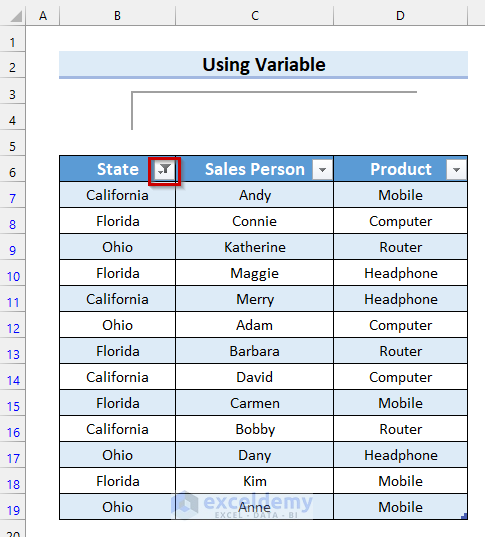
Example 2 – Creating a Search Box in Excel VBA by Using a Variable

Steps:

Insert a Text Box and link it to a cell by following Example 1.
Double-click on the Text Box.

A Module will open with a Private Sub on it.
Paste the following code in that Module.

Private Sub TextBox1_Change()
Dim search_str As String
search_str = "*" & [c4] & "*"
Debug.Print search_str
ActiveSheet.ListObjects("DeclaringVariable_Data").Range.AutoFilter _
field:=1, _
Criteria1:=search_str, _
Operator:=xlFilterValues
End Sub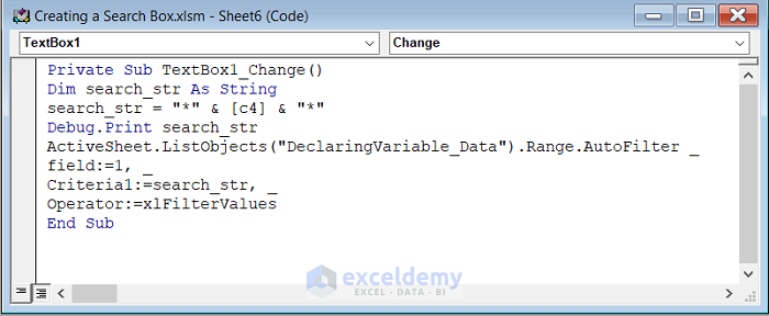

Code Breakdown

A Private Sub Procedure was already created by the Text Box. A Private Sub is only applicable for that specific sheet it is on.
We declared a variable named search_str as String.
We set search_str as “*” & [c4] & “*”.
We used the ListObjects property to return the table named “DeclaringVariable_Data” from the ActiveSheet.
We used the Range.AutoFilter method to filter the range. We selected 1 for the field which will filter the 1st column of the table and we selected search_str as Criteria1 which will match the letter from the 1st column with the input in the search box. For Operator, we selected xlFilterValues which will filter the values.

Save the code and go back to your worksheet.
You will see a filter is added to the column named State.

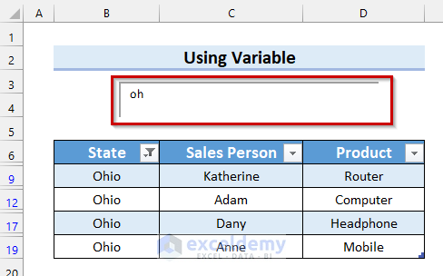
You can search via the search box. We searched for “oh”, and the States that contains “oh” appeared.

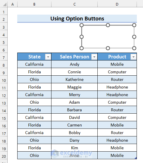
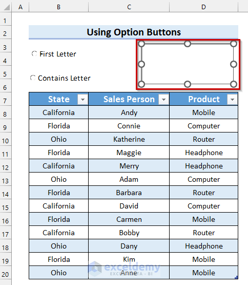
Example 3 – Using a Text Box with Option Buttons

We will create a Search Box in Excel with VBA with two Option Buttons to search for 2 different properties. One will filter if the value contains the searched letter and the other will filter if the searched letter matches the first letter of the value.

Steps:

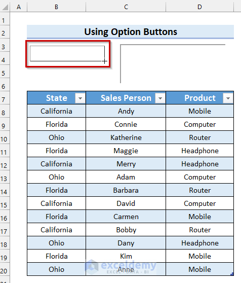
Insert a Text Box and link it to a cell by following the procedure from Example 1.

Go to the Developer tab.
Select Insert.
Select the Option Button from ActiveX Controls.

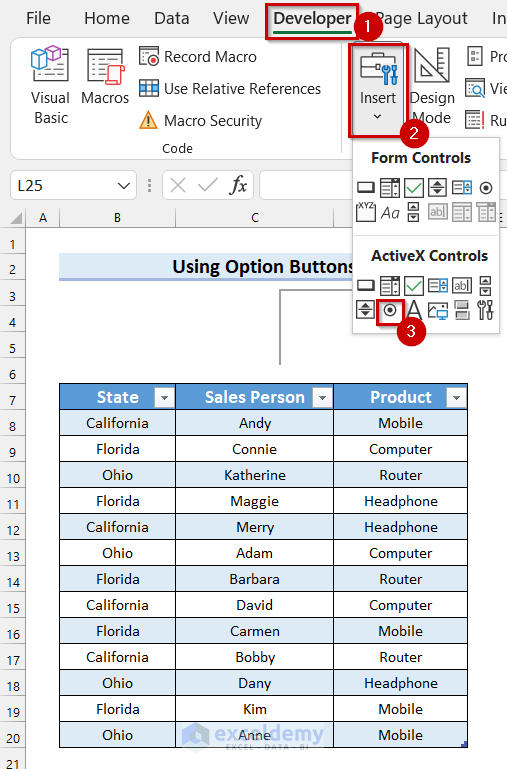
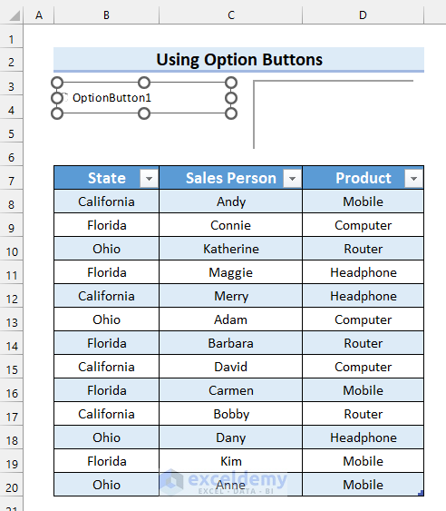
Click and drag your mouse cursor where you want the Option Button.

You will see an Option Button inserted into your Excel sheet.

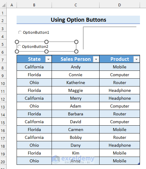
Insert another Option Button in the same way.

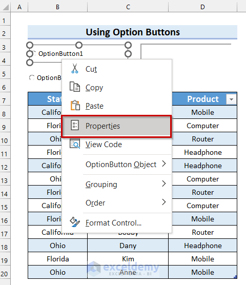
Right-click on the Option Button.
Select Properties.

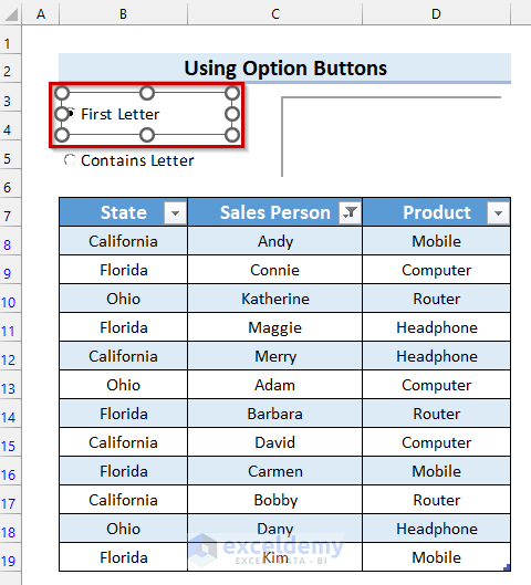
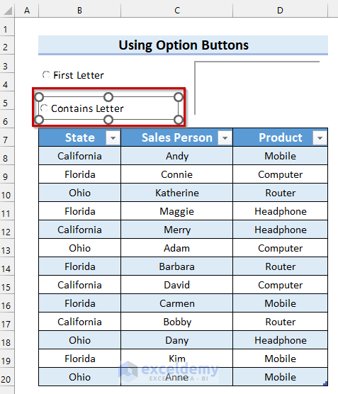
Write the Caption as you want it. We changed it to First Letter.

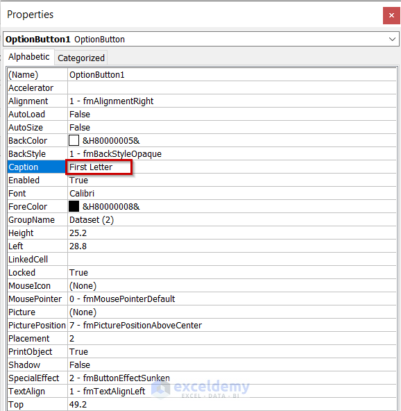
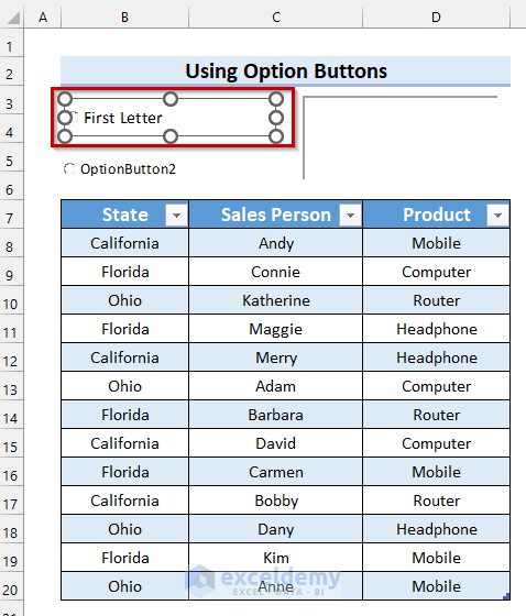
You can see the Caption has changed.

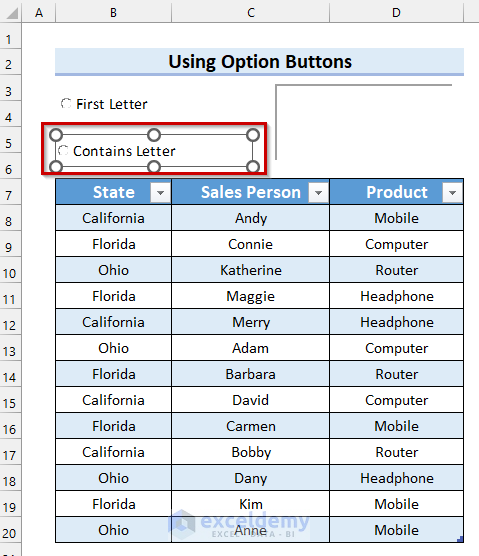
Change the caption of the other Option Button in the same way. We changed it to Contains Letter.

Double-click on the Text Box.

A Module will open with a Private Sub on it.

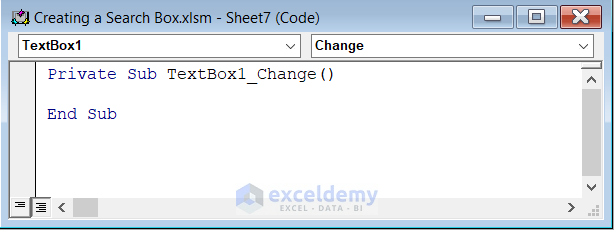
Copy the following code in the Module.

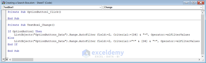
Private Sub TextBox1_Change()
If OptionButton1 Then
    ListObjects("OptionButtons_Data").Range.AutoFilter field:=2, Criteria1:=[D4] & "*", Operator:=xlFilterValues
Else
    ListObjects("OptionButtons_Data").Range.AutoFilter field:=2, Criteria1:="*" & [D4] & "*", Operator:=xlFilterValues
End If
End Sub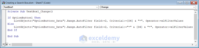

Code Breakdown

A Private Sub Procedure was already created by the text box. A Private Sub is only applicable for that specific sheet it is on.
We used the IF Statement to give different results in two different situations. If OptionButton1 is selected, then Criteria1 is selected as [D4] & “*” for the Range.AutoFilter method. This means it will filter the values that start with the searched letter. Otherwise, Criteria1 of “*” & [D4] & “*” uses the Range.AutoFilter method. That means it will filter the values that contain the searched letter.

Save the code and go back to your worksheet.
Double-click on the Option Button.

Another Private Sub Procedure will be created in the same Module.

Use the following code in the Module.

Private Sub OptionButton1_Click()
Call TextBox1_Change
End Sub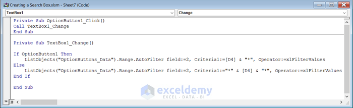

Code Breakdown

A Private Sub Procedure was already created by the OptionButton1. A Private Sub is only applicable for that specific sheet it is on.
We used the Call statement to call the Sub Procedure named TextBox1_Change.

Save the code and go back to your worksheet again.
Double-click on the Option Button named Contains Letter.

Another Private Sub Procedure will be created in the same Module.

Use the following code in the Module.

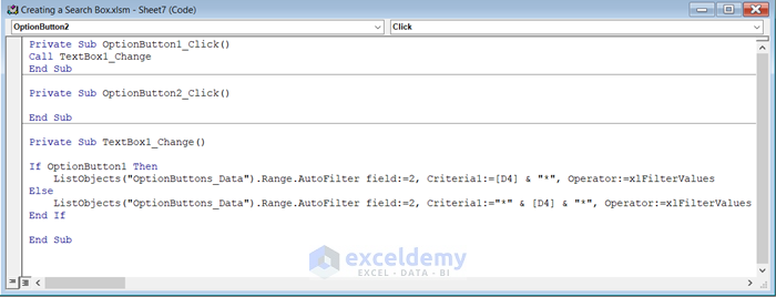
Private Sub OptionButton2_Click()
Call TextBox1_Change
End Sub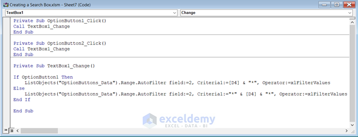

Code Breakdown

A Private Sub Procedure was already created by OptionButton2. A Private Sub is only applicable for that specific sheet it is on.
We used the Call statement to call the Sub Procedure named TextBox1_Change.

Save the code and return to your worksheet.
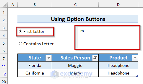
You can use the search box and select your preferred Option Button. We searched for the letter “m” and selected the First Letter. The names that start with “m” are filtered.

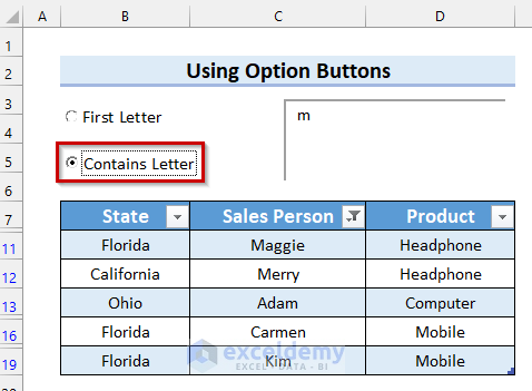
We selected the Option Button named Contains Letter and the names that contain the letter “m” are filtered.

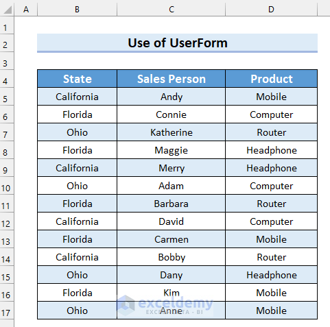
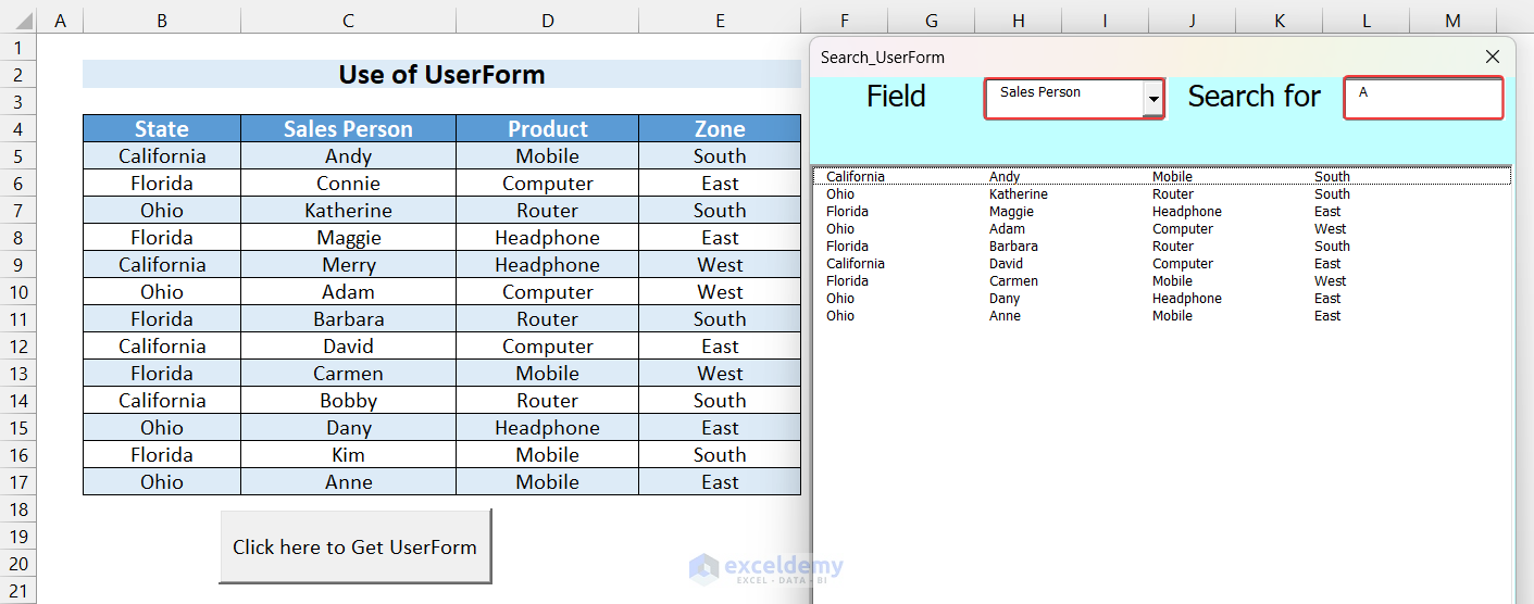
Example 4 – Use the VBA UserForm to Create a Search Box

We’ll use the following dataset which is not a table but a range of data.

Step 1 – Creating and Modifying the UserForm

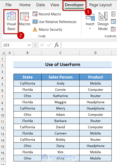
Go to the Developer tab.
Select Visual Basic.

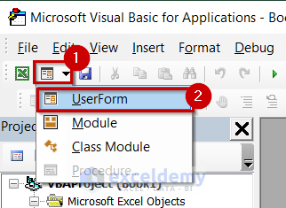
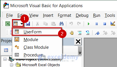
The Visual Basic window will open.
Click on the drop-down menu for UserForm.
Select UserForm.

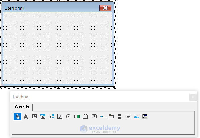
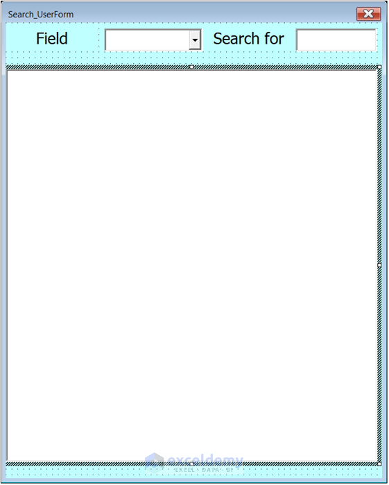
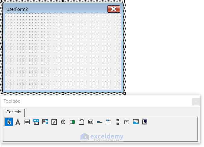
A UserForm will appear.

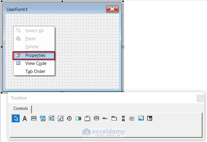
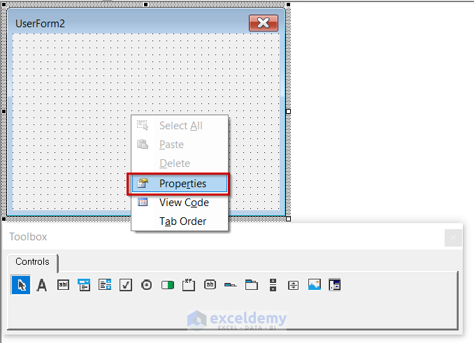
Right-click on the UserForm.
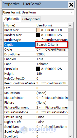
Select Properties.

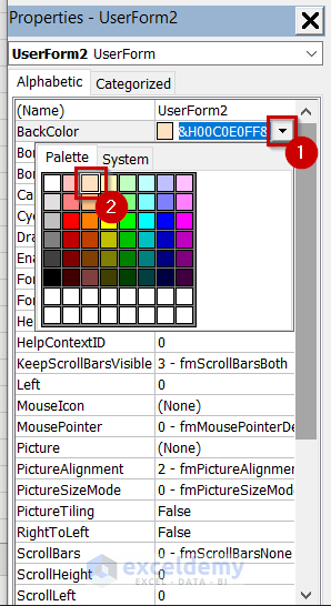
Properties for UserForm1 will appear on the left side of the screen.
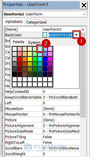
Select the drop-down option from BackColor.
Select the color you want for your background color.

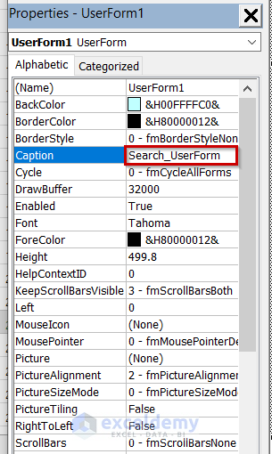
Change the Caption if you want. We changed it to search_UserForm.

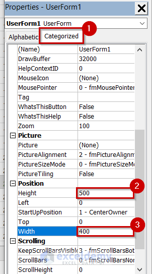
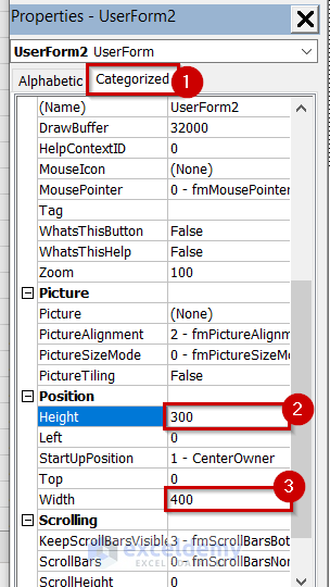
Go to the Categorized tab.
Change the Height as per your preference.
Change the Width as per your preference.

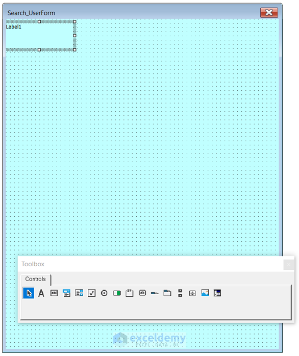
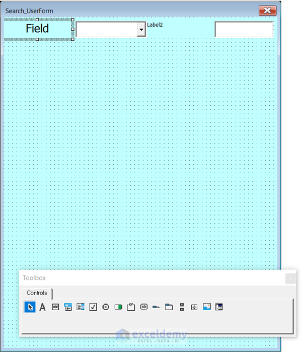
Select Label from the Toolbox.
Click and drag your mouse cursor where you want the Label.

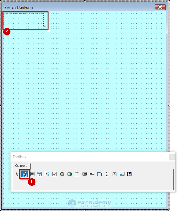
You will see the Label is inserted.

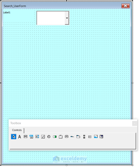
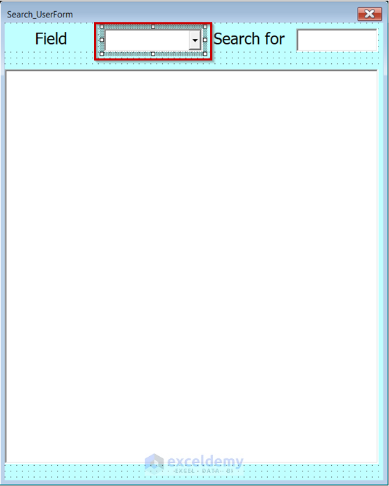
Select a ComboBox from the Toolbox.

Click and drag your mouse cursor where you want your ComboBox.

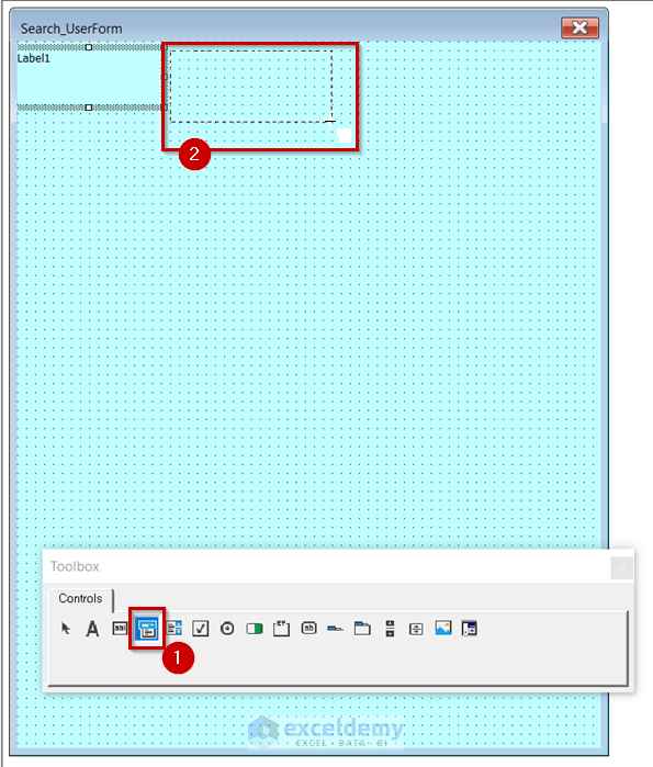
You can see the ComboBox is inserted into the UserForm.

Select Label from Toolbox again.

Click and drag your mouse cursor where you want the Label.

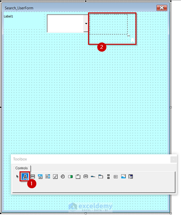
You will see the Label is inserted.

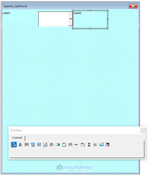
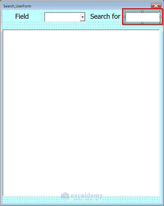
Select a TextBox from the Toolbox.

Click and drag your mouse cursor where you want the TextBox.

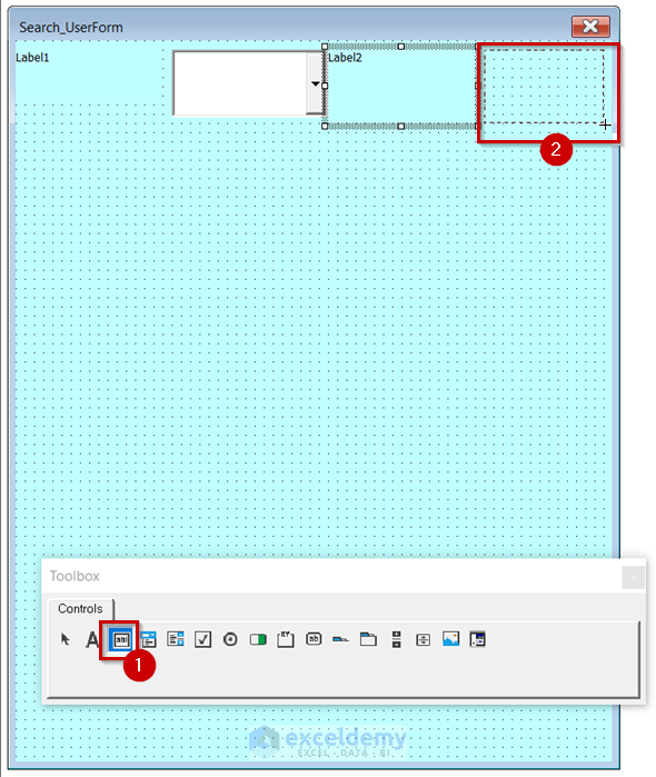
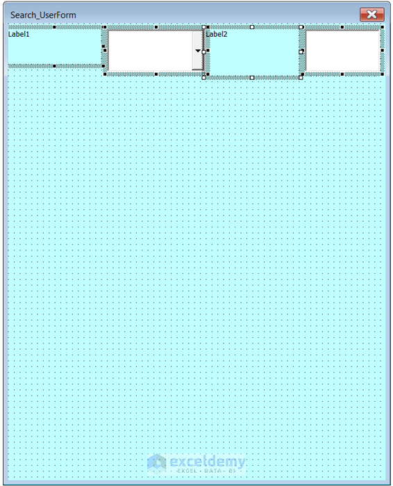
You will see that TextBox is inserted into the UserForm.

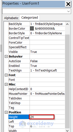
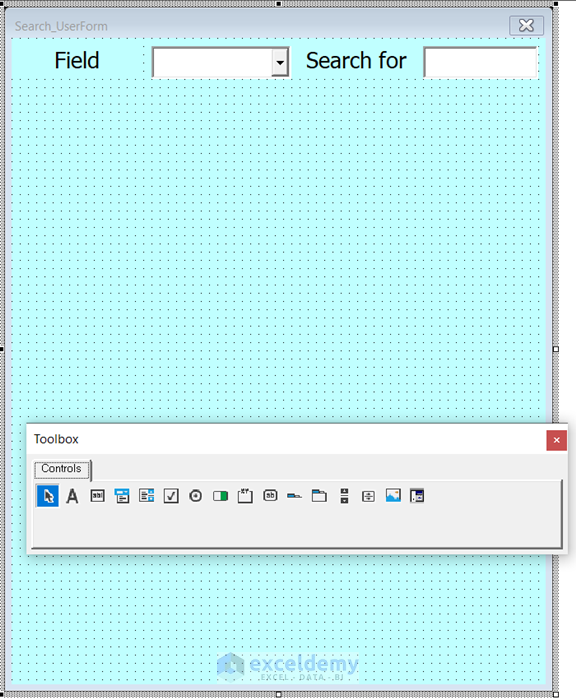
Select all 4 of them together.

Change the Height from Properties as you want. We changed it to 24.

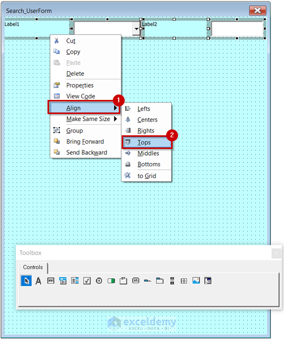
Right-click on any of the boxes.
Select Align.
Select Tops.

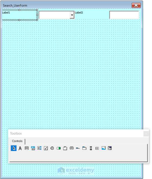
All of the boxes have the same height and they are aligned at the top of the sheet.
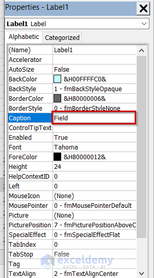
Select Label1.

Change the Caption from the Properties. We changed it to Field.

Click on the drop-down option for Font.

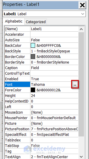
A dialog box will appear.
Choose a Font Size as you want.
You can also change the Font and Font Style from here.
Select OK.

Click on the drop-down option for TextAlign.
Choose fmTextAlignCenter from the drop-down menu.

You can see the caption of Label1 has changed.

Change the Caption of Label2 in the same way.

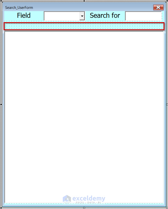
Select ListBox from the Toolbox.

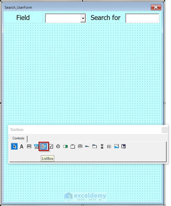
Click and drag the mouse cursor where you want the ListBox.

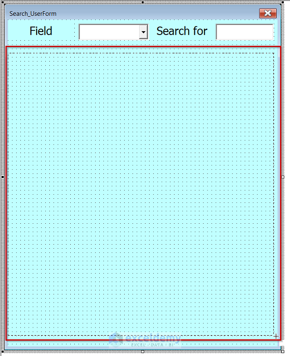
We have inserted everything needed in the UserForm.

Step 2 – Using the VBA Code

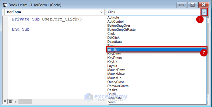
Double-click anywhere in the UserForm.

A module for UserForm1 will open with a Private Sub Procedure on it.
Click on the marked drop-down option on the top-right.
Select Initialize.

Delete the first Private Sub Procedure.
Use the following code in the UserForm.

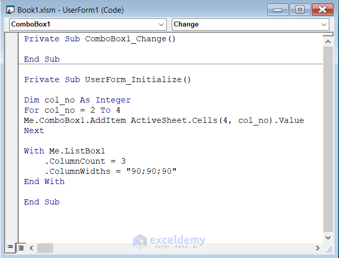
Private Sub UserForm_Initialize()
Dim col_no As Integer

For col_no = 2 To 4
Me.ComboBox1.AddItem ActiveSheet.Cells(4, col_no).Value
Next

With Me.ListBox1
    .ColumnCount = 3
    .ColumnWidths = "90;90;90"
End With

End Sub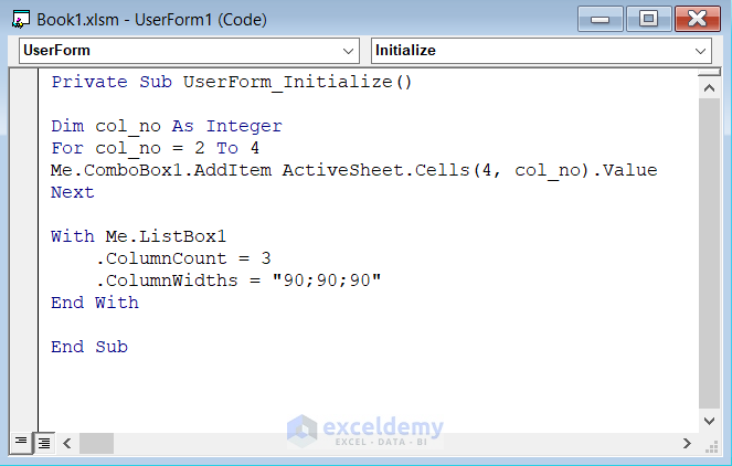

Code Breakdown

A Private Sub Procedure was already created by the UserForm. A Private Sub is only applicable for that specific sheet it is on.
We declared a variable named col_no as an Integer.
We used a For Next Loop to go through columns 2 to 4.
We used the Me keyword to make it behave like an implicitly declared variable. We used the ComboBox1.AddItem method to add the headers of the table to the ComboBox.
We used a With Statement to define the ColumnCount and ColumnWidths in the ListBox1.

Save the code and go back to the UserForm.
Double-click on the ComboBox.

Another Private Sub will be created in the UserForm.

Use the following code in the UserForm.

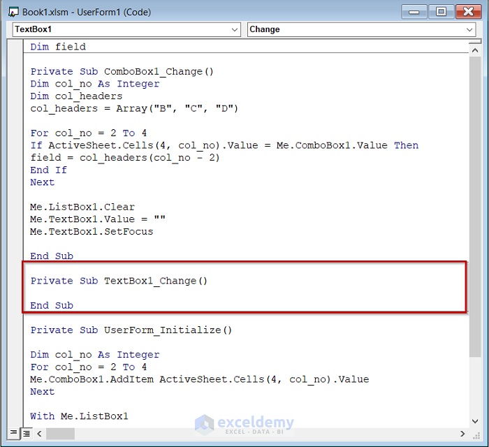
Dim field

Private Sub ComboBox1_Change()
Dim col_no As Integer
Dim col_headers
col_headers = Array("B", "C", "D")

For col_no = 2 To 4
If ActiveSheet.Cells(4, col_no).Value = Me.ComboBox1.Value Then
field = col_headers(col_no - 2)
End If
Next

Me.ListBox1.Clear
Me.TextBox1.Value = ""
Me.TextBox1.SetFocus

End Sub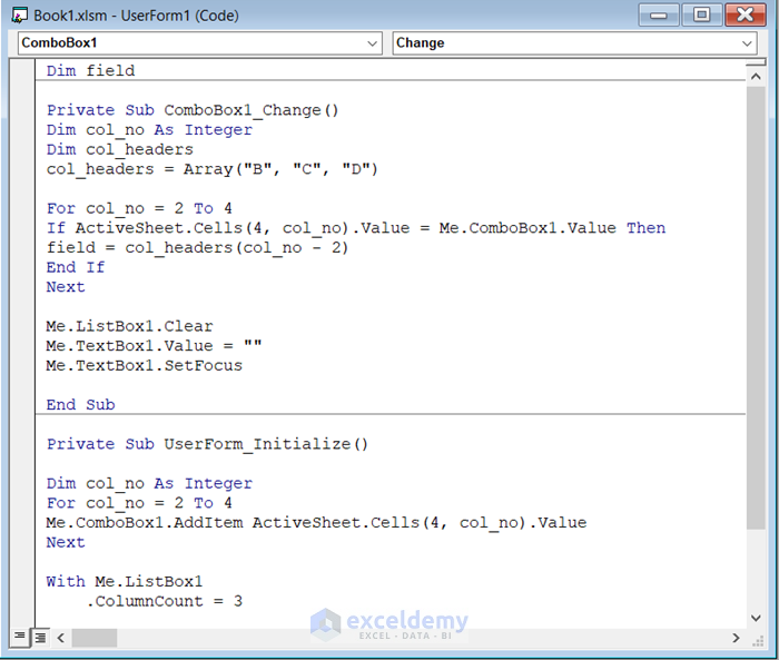

Code Breakdown

We declared a variable named Field.
A Private Sub Procedure was already created by the UserForm. A Private Sub is only applicable for that specific sheet it is on.
We declared a variable named col_no as Integer.
We declared another variable named col_headers.
We used the Array function to assign an array as col_headers.
We used a For Next Loop to go through columns 2 to 4.
We used an IF statement to check if the value in the cell matches the value in ComboBox1. If it matches, then the statement will return the field as col_headers(col_no – 2) which will be the column that will be filtered.
We used ListBox1.Clear to remove all data from ListBox1. We used the Me keyword to make it behave like an implicitly declared variable.
We used TextBox1.Value to specify the text in the text box, and Set it as blank. We also used the Me keyword to make it behave like an implicitly declared variable.
We used TextBox1.SetFocus method to move focus to this specified form.

Save the code and return back to the UserForm.
Double-click on the TextBox.

Another Private Sub Procedure will be created.

Use the following code in the UserForm.

Private Sub TextBox1_Change()
On Error Resume Next

If Me.TextBox1.Text = "" Then
Me.ListBox1.Clear
Exit Sub
End If

Me.ListBox1.Clear
Dim row_no As Integer
Dim last_row_no As Integer
last_row_no = ActiveSheet.Range("B100").End(xlUp).Row

For row_no = 5 To last_row_no
    letter = Len(Me.TextBox1.Text)
    If UCase(Left(ActiveSheet.Cells(row_no, field).Value, letter)) = UCase(Me.TextBox1.Text) Then
    With Me.ListBox1
    .AddItem ActiveSheet.Cells(row_no, "B").Value
    .List(.ListCount - 1, 1) = ActiveSheet.Cells(row_no, "C").Value
    .List(.ListCount - 1, 2) = ActiveSheet.Cells(row_no, "D").Value
    End With
    End If
Next

End Sub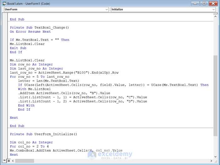

Code Breakdown

A Private Sub Procedure was already created by the UserForm. A Private Sub is only applicable for that specific sheet it is on.
We wrote On Error Resume Next to continue to code if any error occurs.
We used an IF statement to check if the TextBox is blank. If it is blank, then the ListBox1 will be cleared.
We declared a variable named row_no as Integer, and another variable named last_row_no as Integer.
We used the Range.End(xlUp) property to find the last non-blank row number.
We used a For Next Loop to go through all the rows in a column.
We used another IF statement to see if the text in the TextBox matches the value in the cell. The Left function will match from the beginning of the text. We used the UCase function to convert the letter to an uppercase letter.
We used the With statement to add the item to the ListBox and make a list with the other 2 columns if the two values match.

Save the code and go back to your worksheet.

Step 3 – Inserting a Command Button

Go to the Developer tab.
Select Insert.
A drop-down menu will appear.
Select CommandButton from ActiveX Controls.

Click and drag your mouse cursor where you want your CommandButton.

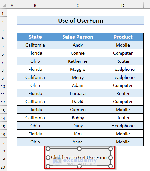
You will see the CommandButton inserted into the worksheet.
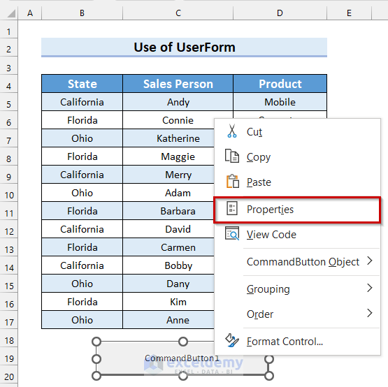
Rght-click on the CommandButton.
Select Properties.

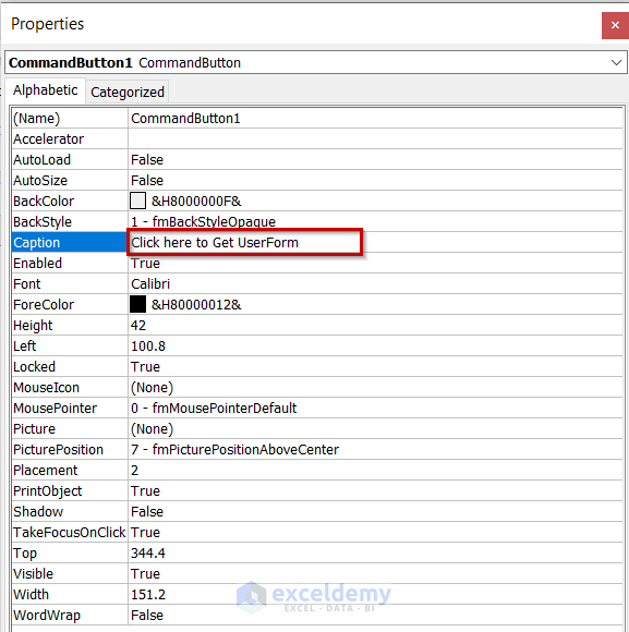
Change the Caption as you want.

Double-click on the CommandButton.

A module will open with a Private Sub on it.
Use the following code in the module.

Private Sub CommandButton1_Click()
UserForm1.Show
End Sub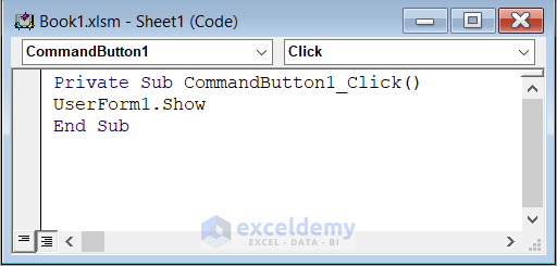

Code Breakdown

A Private Sub Procedure was already created by the CommandButton. A Private Sub is only applicable for that specific sheet it is on.
We used the Show method to display the UserForm1.

Save the code and go back to your worksheet.

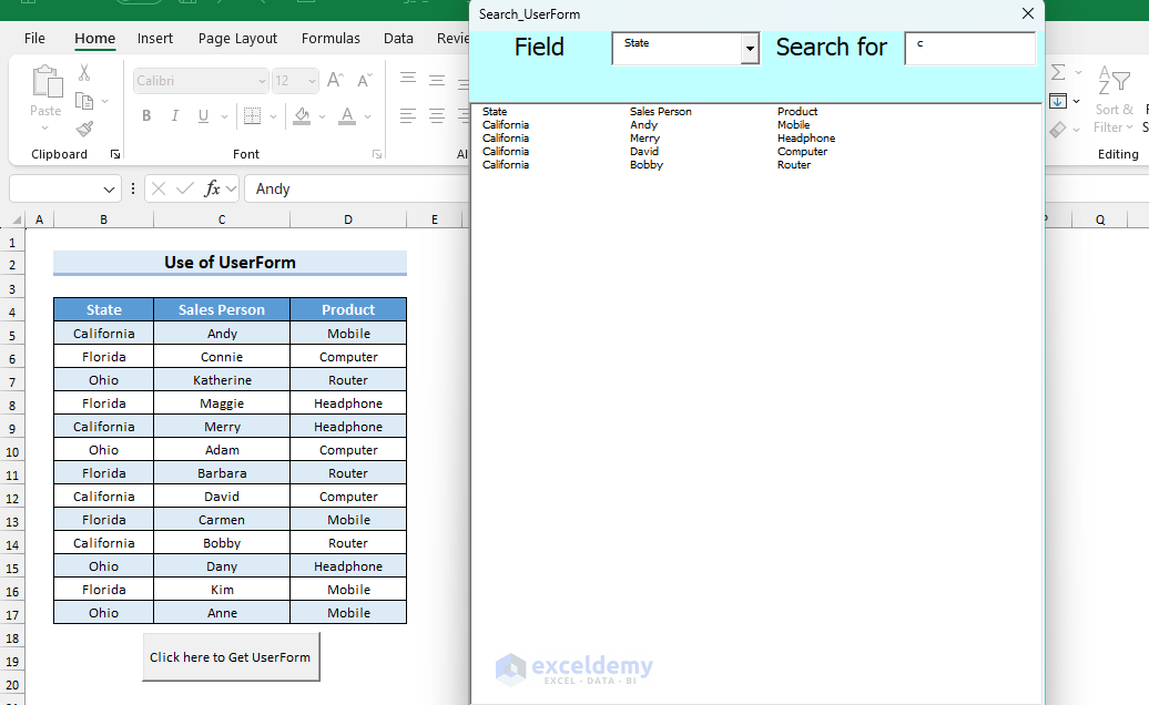
Step 4 – Using the Search Box

Click on the CommandButton.

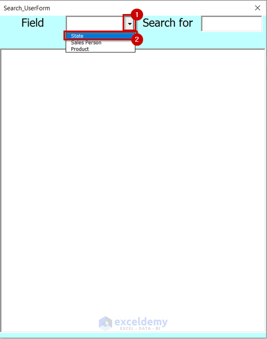
The UserForm will appear.
Select the drop-down option for selecting a Field.
Select the Field from the drop-down menu. We selected State.

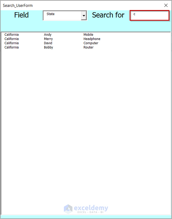
Search for whatever you want. We searched for “c” and the States that start with “c” have appeared.

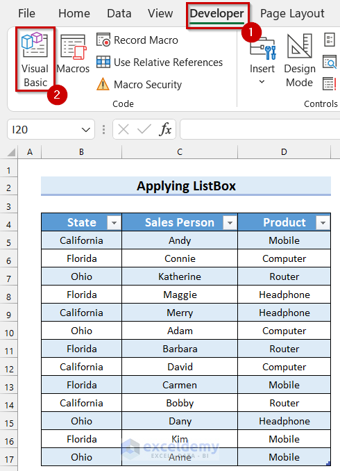
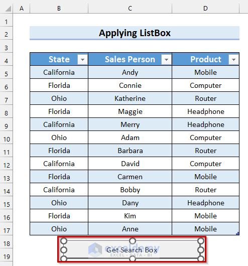
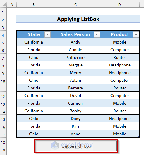
Example 5 – Applying a ListBox to Create a Search Box

Steps:

Go to the Developer tab.
Select Visual Basic.

The Visual Basic window will open.
Click on the drop-down menu for UserForm.
Select UserForm.

A UserForm will appear.

Right-click on the UserForm.
Select Properties.

Properties for UserForm2 will appear on the left side of the screen. Change the BackColor of the UserForm.

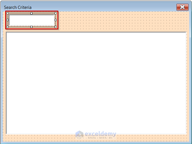
Change the Caption if you want. We changed it to Search Criteria.

Go to the Categorized tab.
Change the Height as per your preference.
Change the Width as per your preference.

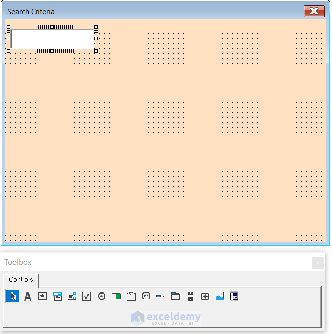
Select TextBox from the Toolbox.

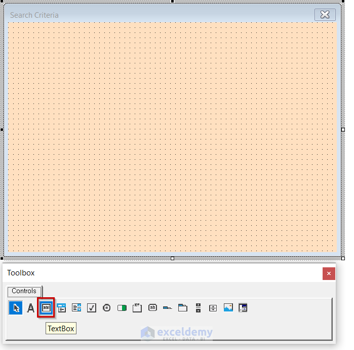
Click and drag your mouse cursor where you want the TextBox.

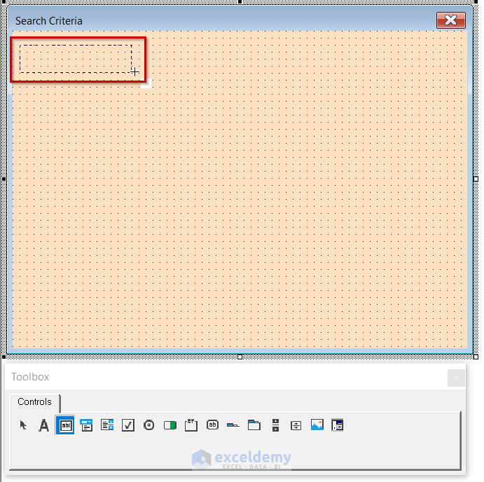
A TextBox is inserted.

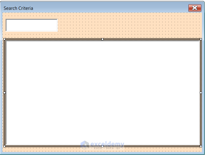
Select ListBox from the Toolbox.
Click and drag the mouse cursor where you want the ListBox.

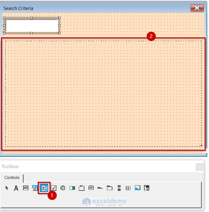
We have inserted everything for the UserForm.

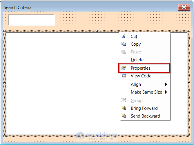
Right-click on the ListBox.
Select Properties.

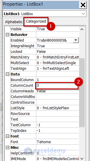
Go to the Categorized tab from the Properties for ListBox1.
Select ColumnCount as your column number in the table. We selected 3 because the table has 3 columns.

Double-click on the TextBox.

A UserForm will open with a Private Sub.
Use the following code in the UserForm.

Private Sub TextBox1_Change()
Dim row_no As Long
Me.TextBox1 = Format(StrConv(Me.TextBox1, vbLowerCase))
Me.ListBox1.Clear
Me.ListBox1.AddItem "Sales Person"
Me.ListBox1.List(0, 1) = "State"
Me.ListBox1.List(0, 2) = "Product"
Me.ListBox1.Selected(0) = True

For row_no = 5 To ActiveSheet.Range("B100").End(xlUp).Row
For sr_for = 1 To Len(ActiveSheet.Cells(row_no, 3))

letter = Me.TextBox1.TextLength
If LCase(Mid(ActiveSheet.Cells(row_no, 3), sr_for, letter)) = Me.TextBox1 And Me.TextBox1 <> "" Then
Me.ListBox1.AddItem ActiveSheet.Cells(row_no, 3)
Me.ListBox1.List(ListBox1.ListCount - 1, 1) = ActiveSheet.Cells(row_no, 2)
Me.ListBox1.List(ListBox1.ListCount - 1, 2) = ActiveSheet.Cells(row_no, 4)
End If

Next sr_for
Next row_no

End Sub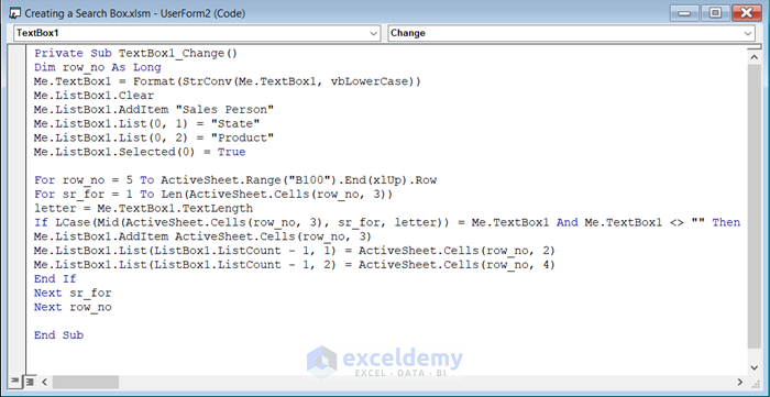

Code Breakdown

A Private Sub Procedure was already created by TextBox. A Private Sub is only applicable for that specific sheet it is on.
We declared a variable named row_no as Long.
We used the Format function to format the text in TextBox. In the Format function, we used the StrConv function to convert the text to lowercase.
We used ListBox1.Clear to remove all data from ListBox1. We used the Me keyword to make it behave like an implicitly declared variable.
We used ListBox1.AddItem to add a new Item to the ListBox, which is the column header of the table.
We used ListBox1.List to get the other two column headers.
We used a For Next Loop to go through all the rows of the table. Another For Next Loop will go through the full length of the string. We used the Len function to return the number of characters.
We used another IF statement to see if the text in the TextBox matches the value in the cell. The Mid function will match from anywhere in the text. We also used the LCase function to convert the letter to a lowercase letter.
We used the ListBox1.AddItem method to add the item to the ListBox if the two values match. We then make a list with the other 2 columns by using ListBox1.List.

Save the code and go back to your worksheet.
Insert a CommandButton by following the procedure from Step 3 of Example 4.
Double-click on the CommandButton.

A module will open with a Private Sub on it.
Use the following code in the module.

Private Sub CommandButton1_Click()
UserForm2.Show
End Sub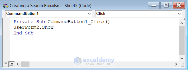

Code Breakdown

A Private Sub Procedure was already created by the CommandButton. A Private Sub is only applicable for that specific sheet it is on.
We used the Show method to display the UserForm2.

Save the code and go back to your worksheet.
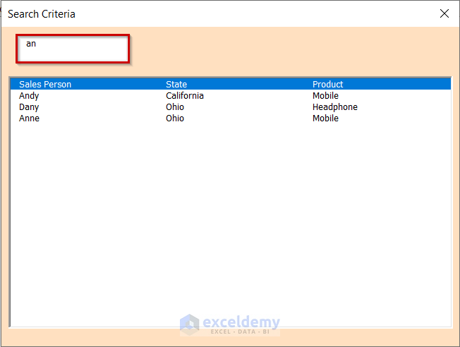
Click on the CommandButton.

The UserForm will open.
You can search for whatever you want. We searched for “an” and the Sales Person names that contain “an” have appeared.

Things to Remember

Whenever working with VBA in Excel, you must save the Excel file as an Excel Macro-Enabled Workbook.

Practice Section

We have provided a practice sheet for you to practice how to create a search box in Excel with VBA.

Download the Practice Workbook

Creating a Search Box.xlsm

<< Go Back to Search Box in Excel | Learn Excel

Get FREE Advanced Excel Exercises with Solutions!

10 Comments

zain Jan 18, 2023 at 11:52 AM

i tried example 5 but it did not work
- Reply
  Mashhura Jan 23, 2023 at 12:54 PM
  
  Hello ZAIN,
  Thanks for your comment. I am replying to you on behalf of ExcelDemy. For Example 5, you will have to keep 2 things in mind.
  1. You will have to change the ColumnCount in the ListBox Properties according to your dataset.
  2. In the VBA code, you will have to change Row and Column numbers according to your dataset.
  I hope this will help you to solve your problem. If it fails to solve your problem, then please specify where are you facing the problem.
  Regards
  Mashhura,
  ExcelDemy.
Robyrubyjane Mar 27, 2023 at 7:35 AM

hi can you make a tutorial that if we put that search box in another sheet than it will find the keyword/data from another sheet?
- Reply
  Zahid Hasan Mar 27, 2023 at 3:31 PM
  Hello ROBYRUBYJANE,
  Thank you for reaching out. If I understand correctly, you are interested in creating a search box that can locate values from another worksheet and transfer them to the current worksheet. To accomplish this, you can use the following steps:
  Begin by creating a search box, and then add the following code to it.
```
Private Sub TextBox1_Change()
    Application.ScreenUpdating = False
    Sheet4.Range("F6:H19").ClearContents
    Sheet4.Range("F6:H19").ClearFormats
    Sheet6.ListObjects("DeclaringVariable_Data").Range.AutoFilter field:=2, Criteria1:=[c4] & "*", Operator:=xlFilterValues
    Sheet6.Range("B6:D19").SpecialCells(xlCellTypeVisible).Copy
    Sheet4.Range("F6").PasteSpecial Paste:=xlPasteAll
    Application.CutCopyMode = False
    Application.ScreenUpdating = True
End Sub
```
  In this scenario, “Sheet4” is the worksheet containing the search box, and any copied values will be pasted into the range B6:D19 of this worksheet. Prior to pasting, the contents and formatting of the destination range will be cleared. “Sheet6” is the worksheet where the specified keyword will be searched for.
  With these steps completed, your search box is now ready for use.
  I hope this helps you to achieve your goal. If you need further assistance in this regard, please let us know.
  
  Regards
  Zahid
  ExcelDemy
Robyrubyjane Mar 27, 2023 at 8:39 AM

hi can i ask how to make a search box that can search data based on date ??
- Reply
  Zahid Hasan Mar 27, 2023 at 3:35 PM
  Hello ROBYRUBYJANE,
  Thank you for your query. To create a search box that will search data based on a provided date, you can follow the steps given below.
  First, construct a search box and add this code to it.
```
Private Sub TextBox1_Change()
    On Error Resume Next
    Application.ScreenUpdating = False
    Sheet9.ListObjects("filter_byDate").Range.AutoFilter field:=1, Criteria1:=">=" & Range("C4").Value, Operator:=xlFilterValues
    Application.ScreenUpdating = True
End Sub
```
  In this code, “Sheet9” refers to the specific worksheet containing the data that requires searching based on dates. The code we have used employs the “greater than or equal” operator, indicating that any data with dates preceding the specified date will not appear in the output.
  I hope this answers your question. If you have any more queries, please please reach out to us.
  
  Regards
  Zahid
  ExcelDemy
john May 26, 2023 at 2:23 PM

What if the range contains not only text but also pictures? Is it still possible to do that?
- Reply
  Mashhura Jahan May 28, 2023 at 12:33 PM
  
  Hi JHON,
  Thanks for your comment. I am replying to you on behalf of ExcelDemy. If you insert pictures with text in the same cell like the following dataset, you will be able to search the pictures easily by following the first method from this article.
  
  In the following image, you can see that the results for the router are displayed with pictures.
  
  For this case, you will have to set the Properties for the pictures as Move and size with cells from the Format Graphic task pane.
  
  I hope this will help you to solve your problem. Please let us know if you have other queries.
  Regards
  Mashhura Jahan
  ExcelDemy.
Tarekzhran Jul 1, 2023 at 4:44 AM

In 04 example how can make listbox on 14 columns and how can search by any contain alphabet first or left and middle
- Reply
  Mursalin Ibne Salehin Jul 3, 2023 at 10:53 AM
  Dear TAREKZHRAN,
  Thank you for your comment. Making a listbox of 14 columns and creating a search box will be complex. However, you can do that easily by modifying the code we provided with ComboBox.
  
  To make a list of 14 columns change the value of col_no variable in the code we have given. Here we set 2 to 4 as col_no. Suppose your column number starts from Column B to Column O, in this case, set col_no as 2 to 15.
  
  In the ComboBox1_Change named subprocedure change the col_header array and col_no variable like below.
```
col_headers = Array("B", "C", "D", "E", "F", "G", "H", "I", "J", "K", "L", "M", "N","O")
For col_no = 2 To 15
```
  Similarly, in UserForm_Initialize named sub procedure set col_no as 2 to 15 and ColumnCount to 14.
  
  To search the alphabet from left or middle or anywhere, we will replace the Left function with the InStr function. The Left function is used to search only for the first alphabet whereas Instr will help you to find it from anywhere in the text. The modified line is below.
```
If InStr(1, UCase(ActiveSheet.Cells(row_no, field).Value), UCase(Me.TextBox1.Text)) > 0
```
  After modifying the code for TextBox1_Change named sub procedure will be like below.
```
Private Sub TextBox1_Change()
On Error Resume Next
If Me.TextBox1.Text = "" Then
Me.ListBox1.Clear
Exit Sub
End If
Me.ListBox1.Clear
Dim row_no As Integer
Dim last_row_no As Integer
last_row_no = ActiveSheet.Range("B100").End(xlUp).Row
For row_no = 5 To last_row_no
	letter = Len(Me.TextBox1.Text)
	If InStr(1, UCase(ActiveSheet.Cells(row_no, field).Value), UCase(Me.TextBox1.Text)) > 0 Then
	With Me.ListBox1
	.AddItem ActiveSheet.Cells(row_no, "B").Value
	.List(.ListCount - 1, 1) = ActiveSheet.Cells(row_no, "C").Value
	.List(.ListCount - 1, 2) = ActiveSheet.Cells(row_no, "D").Value
	End With
	End If
Next
End Sub
```
  After applying the code, you will get results like the picture below.
  
  The Excel file of the solution is attached below. You can download and use it.
  Answer.xlsm
  Hope this will help you to solve your problem. Please let us know if you have other queries.
  Regards,
  Mursalin
  ExcelDemy.

Create a Search Box in Excel with VBA (5 Suitable Examples)

Example 1 – Using the Text Box Feature to Create a Search Box in Excel

Example 2 – Creating a Search Box in Excel VBA by Using a Variable

Example 3 – Using a Text Box with Option Buttons

Example 4 – Use the VBA UserForm to Create a Search Box

Step 1 – Creating and Modifying the UserForm

Step 2 – Using the VBA Code

Step 3 – Inserting a Command Button

Step 4 – Using the Search Box

Example 5 – Applying a ListBox to Create a Search Box

Things to Remember

Practice Section

Related Articles

Leave a reply Cancel reply