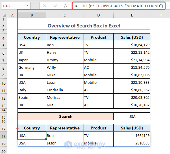
Here’s an overview of implementing a search box via the FILTER function.
Download the Practice Workbook
How to Create a Search Box in Excel – 3 Methods
Method 1 – Conditional Formatting to Highlight Searched Data
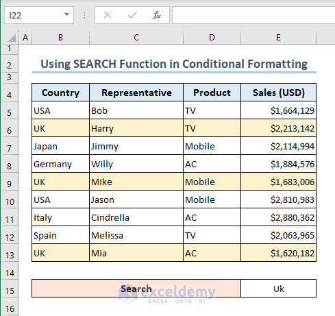
Case 1.1 – Using the SEARCH Function in Conditional Formatting
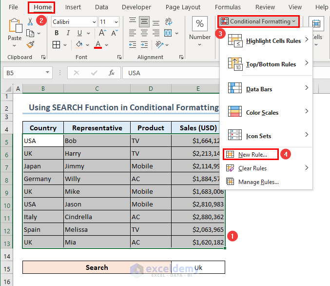
- Go to the Home tab.
- Expand the Conditional Formatting command.
- Click on the New Rule option.
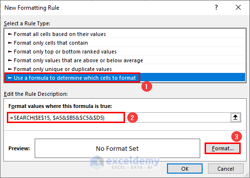
- Select the Use a formula to determine which cells to format option from the Select a Rule Type field.
- Insert the following formula in the formula bar.
=SEARCH($E$15, $A5&$B5&$C5&$D5)
$E$15 = UK = Lookup value and $A5&$B5&$C5&$D5 is the range A5:D5 where to search for matches and highlight.
- Click on the Format button.
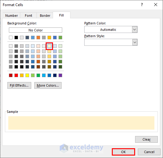
- Select the background color.
- Press the OK button.
- Press OK again.
- Excel highlights the data containing UK in the B5:E13 range after inputting UK in the E15 cell.
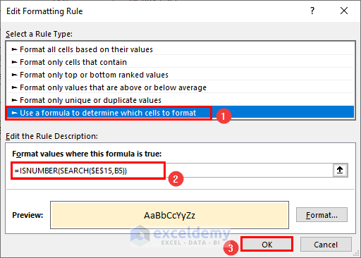
Case 1.2 – Inserting the ISNUMBER Function in Conditional Formatting
- Select the Use a formula to determine which cells to format option from the Select a Rule Type field of the Edit Formatting dialog.
- Insert the following formula in the formula bar and click on OK:
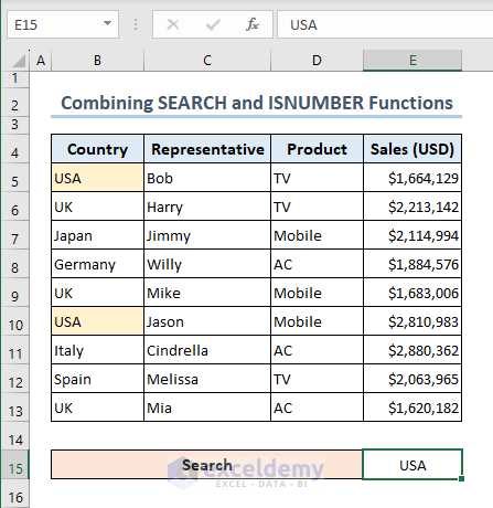
=ISNUMBER(SEARCH($E$15,B5))
E15 = USA matches with the B5 and the rest of the cells accordingly.
- We get the gold-highlighted data containing USA in the B5:E13 range after typing USA in the E15 cell.
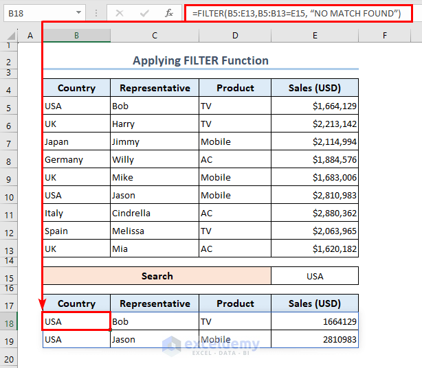
Method 2 – Use the Excel FILTER Function to Create a Search Box
- Put a search term in cell E15.
- Applying the following formula in B18:
=FILTER(B5:E13,B5:B13=E15, “NO MATCH FOUND”)
E15 = USA matches with the B5:B13 range and picks data from B5:E13 = Array range.
The FILTER function is only available on Microsoft 365, Excel 2021, and Excel 2019 versions.
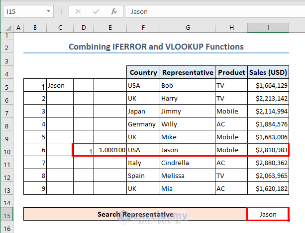
Method 3 – Search Box Formula Using IFERROR and VLOOKUP Functions
- We moved the dataset four columns to the right (to F:I).
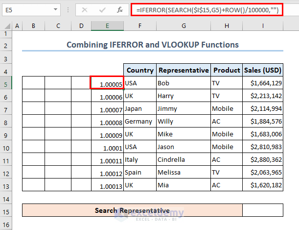
- Insert the following formula in the E5 cell to assign a numerical value:
=IFERROR(SEARCH($I$15,G5)+ROW()/100000,"")
From the E5 cell, ROW() = 5 thus ROW()/100000 = 0.00005 and SEARCH($I$15,G5) = 1. Therefore, IFERROR(SEARCH($I$15,G5)+ROW()/100000,””) = 1.00005 since the IFERROR function prevents errors.
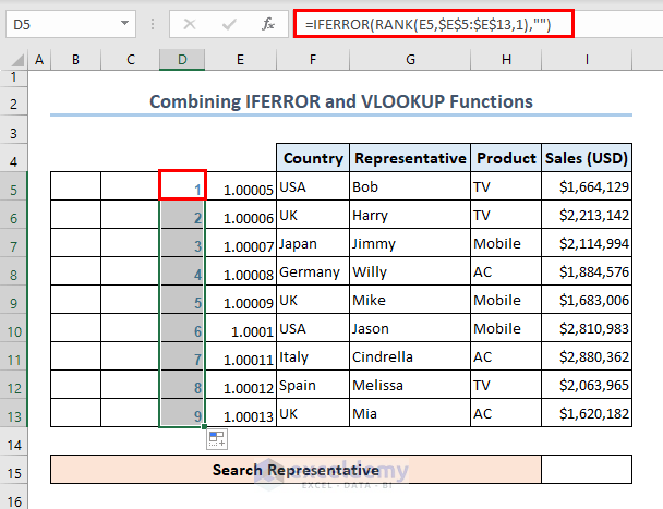
- Apply the following formula in the D5 cell:
=IFERROR(RANK(E5,$E$5:$E$13,1),"")
The RANK function organizes data in ascending order. E5 = 1.00005 is the lowest in the E5:E13 range therefore it outputs 1 in the D5 cell.
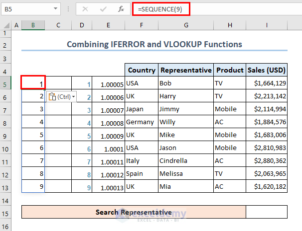
- Insert the following formula in the B5 cell:
=SEQUENCE(9)
- Apply the following formula in the C5:C13 range:
=IFERROR(VLOOKUP(B5,$D$5:$G$13,4,FALSE),"")
The VLOOKUP function looks for the B5 from the D5:G13 range. 4 means the 4th column = Column G of the D5:G13 range and FALSE for the exact match.
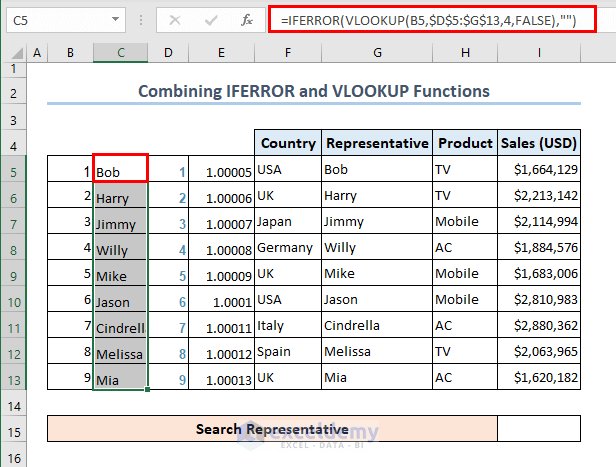
- We obtain the information of representative Jason in the 10th row once we type Jason in the I15 cell.
How to Create a Filtering Search Box in Excel
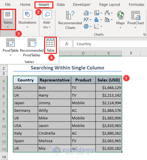
Method 1 – Search Within a Single Column
- Select the B4:E13 range.
- Go to the Insert menu.
- Click on the Table command.
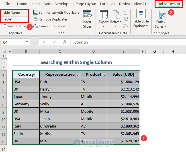
- Select the table and go to the Table Design tab, then rename it as Table1 in the Table Name field.
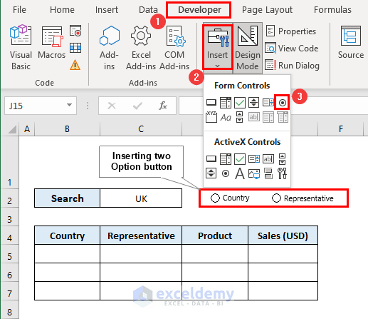
- Go to the Developer tab.
- Click on the Insert command.
- Select the Option button.
- We inserted two buttons for Country and Representative.
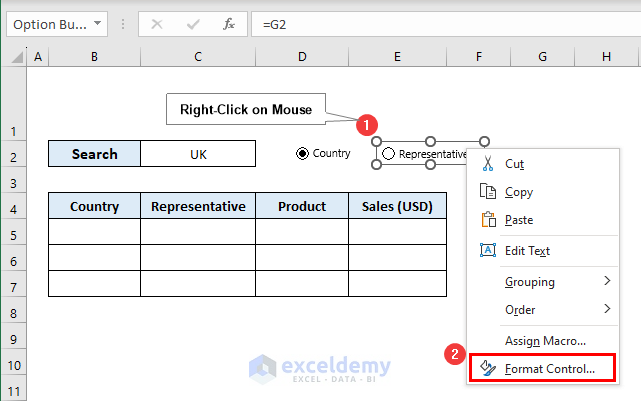
- Select the Option button and right-click on it.
- Click on the Format Control option from the context menu.
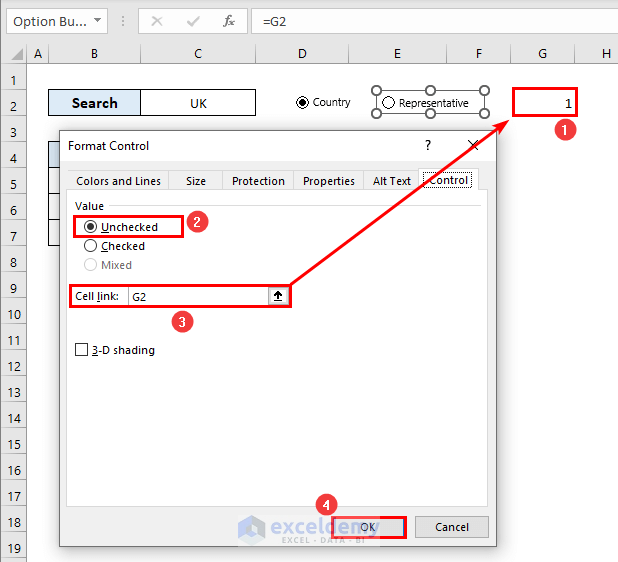
- In the Format Control dialog box, select Unchecked from the Value.
- Insert 1 in the G2 cell.
- Type G2 in the Cell Link field.
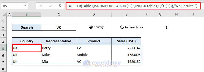
- Insert the following formula in the C2 cell:
=FILTER(Table1,ISNUMBER(SEARCH($C$2,INDEX(Table1,0,$G$2))),"No Results!")
Formula Breakdown
- INDEX function catches all the countries’ names from Table1.
- SEARCH function figures out C2 = UK from Table1 Thus it returns 1 for each match.
- ISNUMBER function converts the 1 into TRUE.
- FILTER function gathers 3 data that output TRUE.
Method 2 – Search Within Multiple Columns
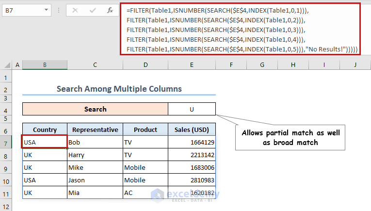
- Insert the formula as follows in the B7 cell:
=FILTER(Table1,ISNUMBER(SEARCH($E$4,INDEX(Table1,0,1))),
FILTER(Table1,ISNUMBER(SEARCH($E$4,INDEX(Table1,0,2))),
FILTER(Table1,ISNUMBER(SEARCH($E$4,INDEX(Table1,0,3))),
FILTER(Table1,ISNUMBER(SEARCH($E$4,INDEX(Table1,0,4))),
FILTER(Table1,ISNUMBER(SEARCH($E$4,INDEX(Table1,0,5))),"No Results!")))))
- We get 5 results for USA and UK after typing U in the E4 cell.
Formula Breakdown
- INDEX function catches all the country, representative, product, and Sales (USD) from Table1. INDEX(Table1,0,1)= range of country, INDEX(Table1,0,2)=range of Representatives, and so on.
- SEARCH function figures out E4 = U from Table1 Thus it returns 1 for each match.
- ISNUMBER function converts the 1 into TRUE.
- FILTER function gathers 5 data that output TRUE.
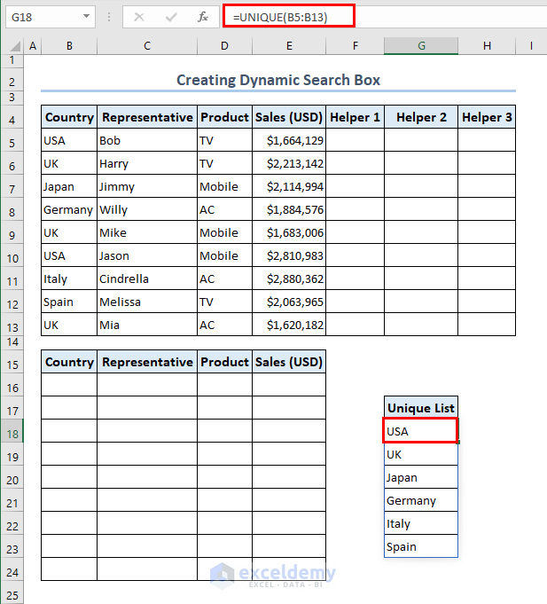
How to Make a Dynamic Search Box in Excel
- Convert the names of countries into a unique list by applying the following formula in G18:
=UNIQUE(B5:B13)
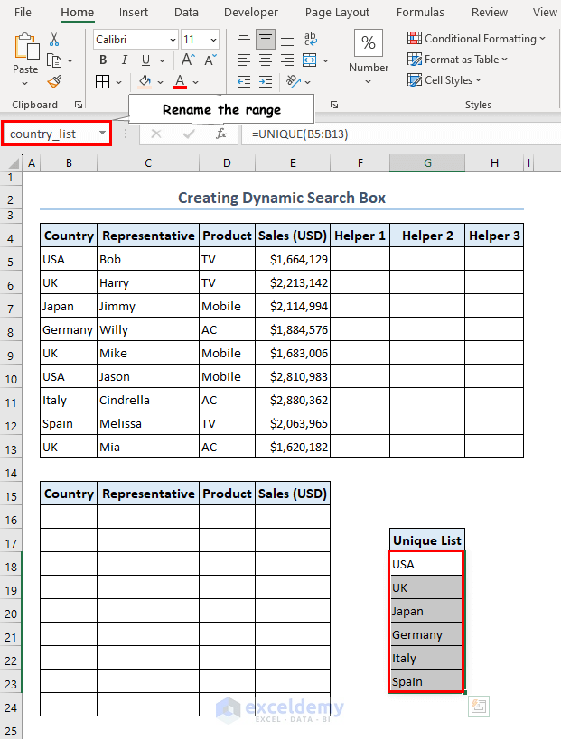
- Select the G18:G23 range and rename it as country_list.
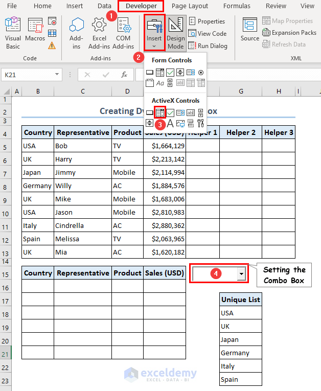
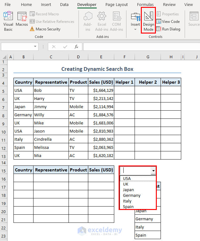
- Go to the Developer tab.
- Expand the Insert option.
- Select the Combo Box and place it into the worksheet.
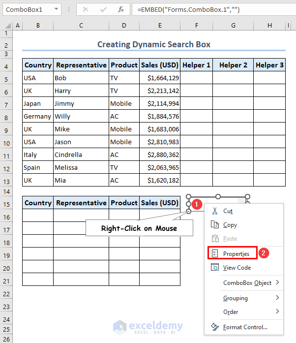
- Right-click on the Combo Box.
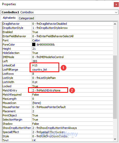
- Click on the Properties from the Context menu list.
- Insert H15 in the LinkedCell field.
- Type country_list in the ListFillRange field.
- Input 2-fmMatchEntryNone in the MatchEntry field.
- Any selection from the drop-down list will be written in the H15 cell.
- Get the dropdown list from the ComboBox by disabling the Design Mode.
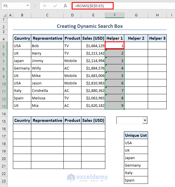
- Inserting the formula below in the F5 cell obtains a serial for the Helper1 column.
=ROWS($E$5:E5)
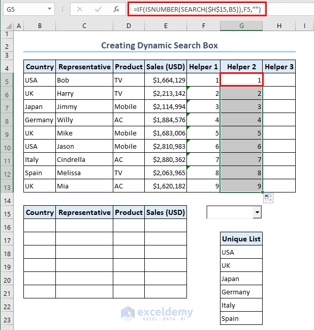
- Insert the following formula in G5 to obtain a serial for the Helper2 column.
=IF(ISNUMBER(SEARCH($H$15,B5)),F5,"")
Formula Breakdown
- SEARCH($H$15,B5) outputs 1 for each match.
- ISNUMBER(SEARCH($H$15,B5)) delivers TRUE for each 1 obtained by the SEARCH function.
- IF function indicates to write the value of the Helper1 column for TRUE.
- Use the following formula in H5 for a serial for the Helper3 column:
=IFERROR(SMALL($G$5:$G$13,F5),"")
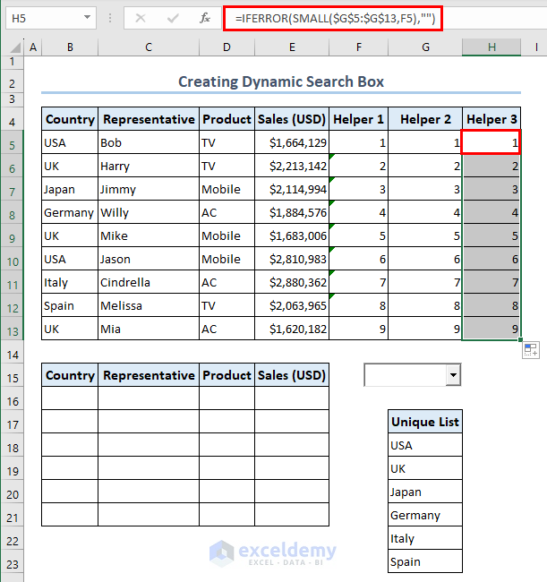
Formula Breakdown
- SMALL($G$5:$G$13,F5) outputs in ascending order. It finds F5 from the G5:G13 range.
- IFERROR function writes the outcome from the SMALL otherwise, leave the cell blank.
- Insert the following formula in B16:
=IFERROR(INDEX($B$5:$E$13,$H5,COLUMNS($I$4:I4)),"")
- Change the values of the drop-down and you’ll get different results.
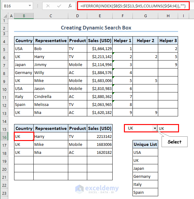
Formula Breakdown
- COLUMNS($I$4:I4) = 1
- INDEX($B$5:$E$13,$H5,COLUMNS($I$4:I4)) = INDEX($B$5:$E$13,2,1) that dictates to pick up the value of B6 cell which contains UK.
- IFERROR writes the value obtained from the result of the INDEX function; otherwise, it leaves blank.
Frequently Asked Questions (FAQs)
Can we use the FIND function instead of the SEARCH function?
It depends on your preference since the FIND function is a case-sensitive function whereas the SEARCH function doesn’t respond to case sensitivity.
Where is the search button in Excel?
You can enable the search button by pressing Ctrl + F keys. However, to search for a text or number from the worksheet, go to the Home menu, expand the Find & Select command, and select Find.
What is the search type in Excel?
The Excel SEARCH function is categorized under string or text functions. However, it delivers an integer output.
Search Box in Excel: Knowledge Hub
- Create a Search Box
- Create a Search Box without VBA
- Create a Filtering Search Box for Your Excel Data
- Create a Search Box for Multiple Sheets
- Create a Search Box with VBA
- Create Search Box in Excel with Conditional Formatting
<< Go Back to Learn Excel
Get FREE Advanced Excel Exercises with Solutions!

That’s formula is Great, thanks to it
Hello Okto,
You are most welcome. Glad to hear that the formula was great to you. We always try to provide the best useful working formulas to ease your works.
Keep learning Excel with ExcelDemy!
Regards
ExcelDemy