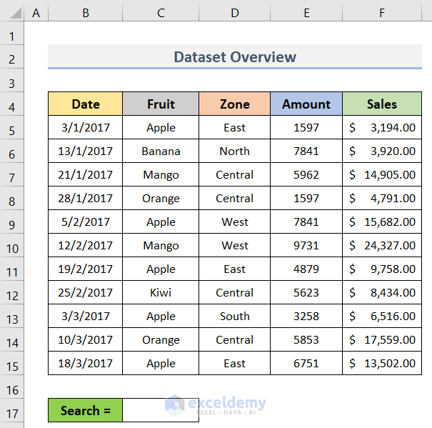
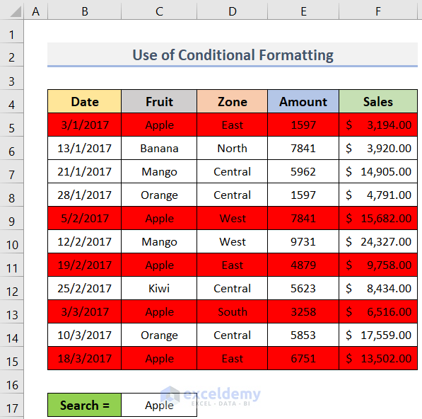
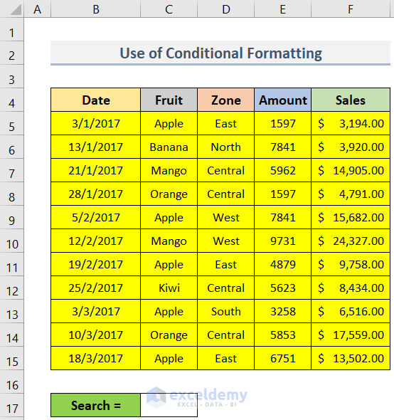
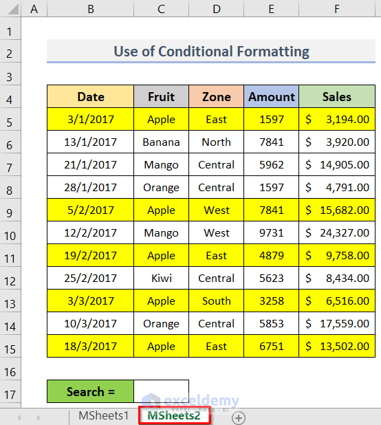
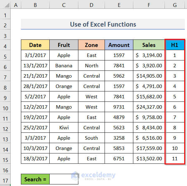
We have a dataset that contains the Dates, Fruit names, Zones, Amounts, and Sales of some orders.
Method 1 – Apply Conditional Formatting to Create a Search Box Without VBA
1.1 Search Box for a Single Excel Worksheet
Steps:
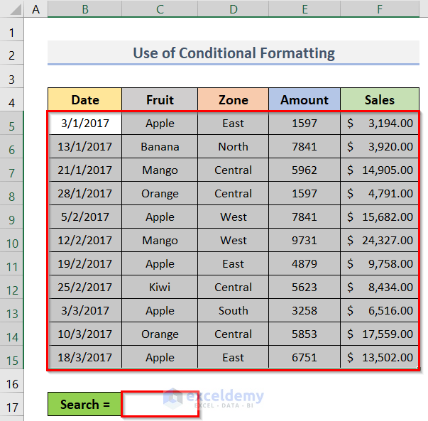
- Go to cell C17 or the cell that will contain the search box.
- Go to the Home tab.
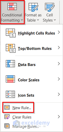
- Click on the Conditional Formatting drop-down menu.
- Select New Rule from the dropdown.
- The New Formatting Rule window will appear.
- Click on Use a formula to determine which cells to format from the Select a Rule Type section.
- Go to the Format values where this formula is true box.
- To insert the Search Box, type the following formula in the box:
=SEARCH($C$17, $B&$C5&$D5&$E5&$F5)- Click on Format to format the searched cell or row to highlight.
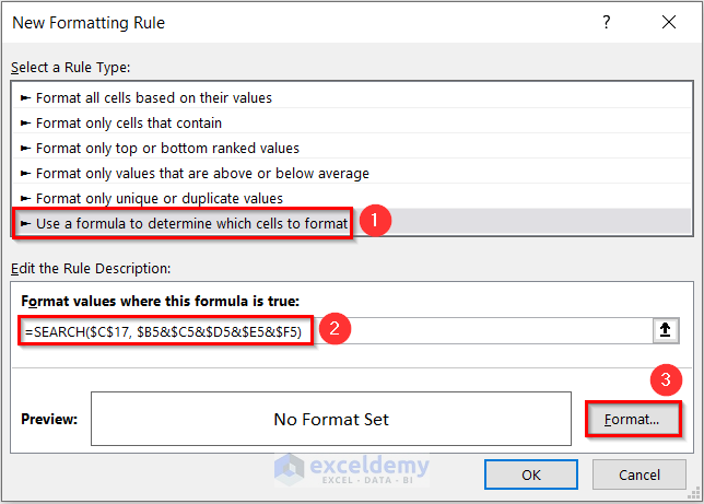
In this formula, $C$17 denotes the location of the search box, and the $ sign is used to lock the cell. However, the B5, C5, D5, E5, and F5 refer to the columns from which the search box will search for the data (text or number).
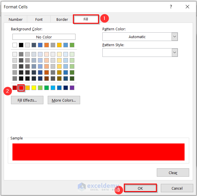
- The Format Cells dialog box will appear.
- We want to highlight the entire row of the searched data from the dataset.
- Go to the Fill tab > Background Color > Select any Color from the list > OK.
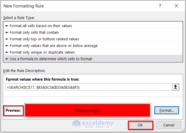
- You will see the New Formatting Rule window again.
- Go to the Preview section and see if it shows the same formatting as you selected.
- Click OK.
You will see the whole dataset B5:F15 (that you entered in the SEARCH function) with the formatting.
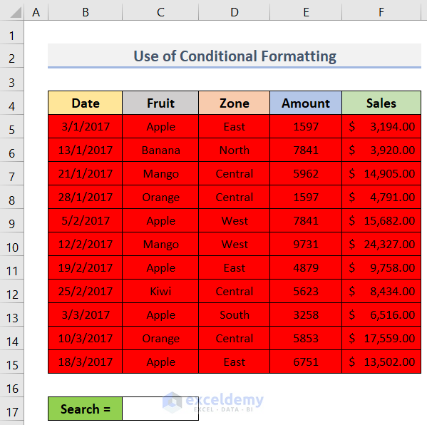
- Type Apple in cell C17.
![]()
Only the rows (5, 9, 11, 13, 15) that contain Apple will remain highlighted with Red color. See the screenshot below.
Read more: How to Create a Search Box in Excel
1.2 Search Box for Multiple Excel Worksheets
Steps:
- Go to the Home tab.

- Click on Conditional Formatting > New Rule.

- The New Formatting Rule window will pop up.
- Go to the Select a Rule Type > Use a formula to determine which cells to format.
- To create the search box, keep the cursor in the Format values where this is true box and enter the following formula:
=SEARCH(MSheets1!$C$17, $B5&$C5&$D5&$E5&$F5)- Click on Format.
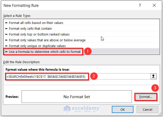
In the formula, MSheets1! refers to the MSheets1 worksheet, where we assign the search box and look for the data.
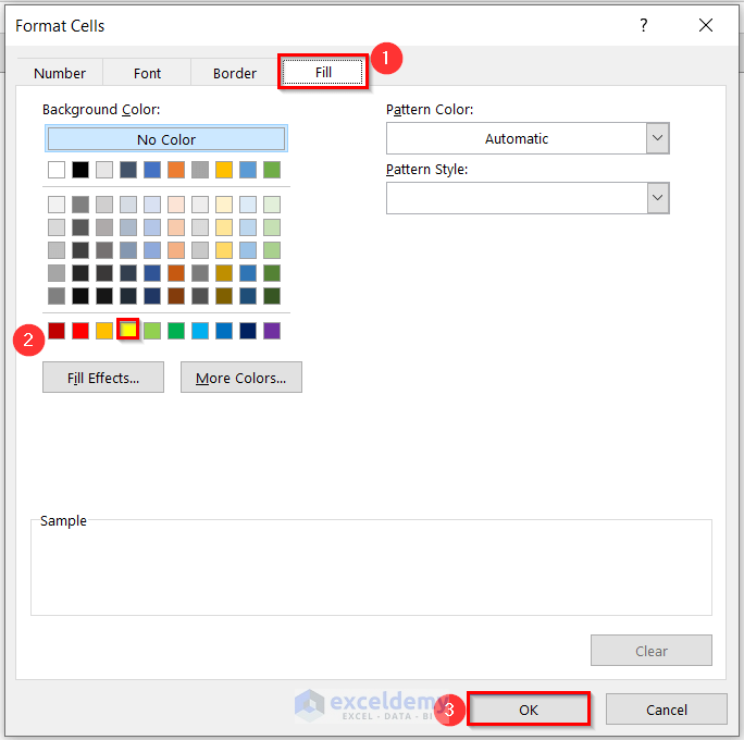
- The Format Cells dialog box will open.
- Go to the Fill tab.
- Go to the background color section and select any color you wish.
- Click on the OK button.
- Check the Preview section to see if the formatting is okay or not.
- If everything is okay, click OK.
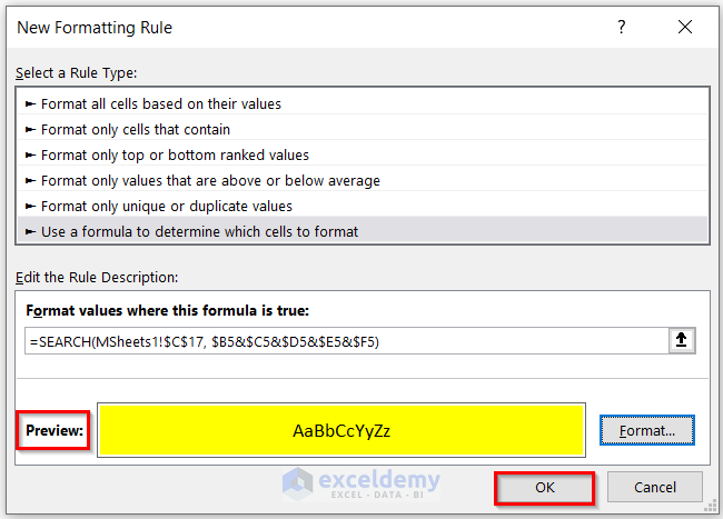
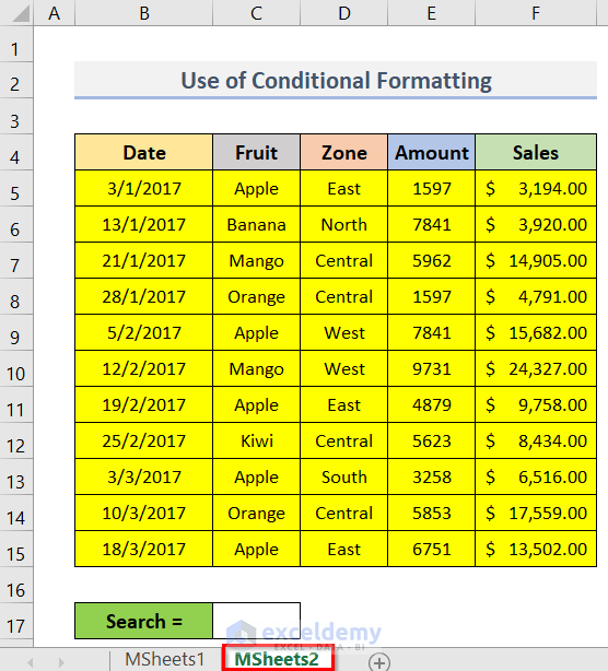
You will see the whole dataset (B5:F15) of the MSheets1 worksheet with the formatting.
- Apply the same Conditional Formatting and SEARCH function to the MSheets2 worksheet.
The MSheets2 will show the same formatting in the whole dataset (B5:F15).
- Go to MSheets1 > cell C17 > type Apple.
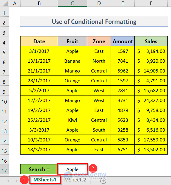
All the rows containing Apple will remain highlighted with Yellow color in the MSheets1 worksheet.
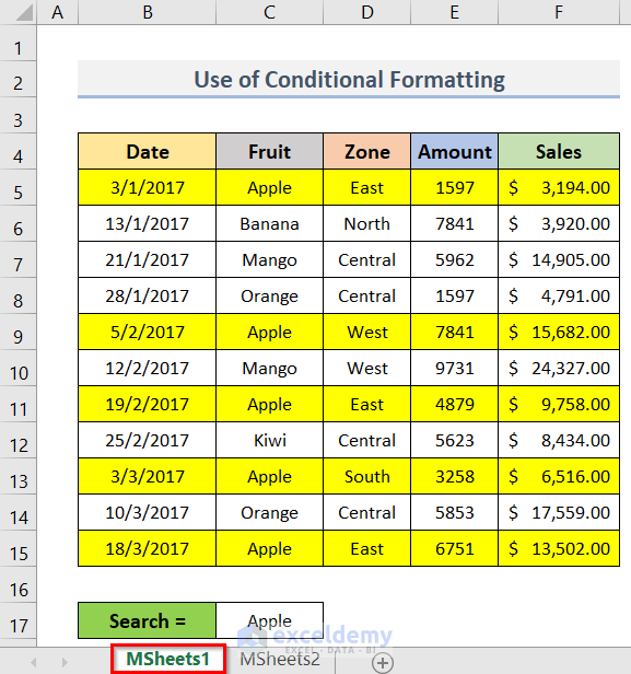
- Go to the MSheets2 worksheet, and you will see the same formatting here.
Method 2 – Create a Dynamic Filter Search Box Without VBA Using Excel Functions
Steps:
- Select the range (C4:C15) from where you want to search the desired data.
- Right-click on the selection and click on Copy.
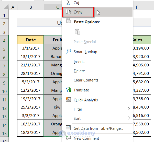
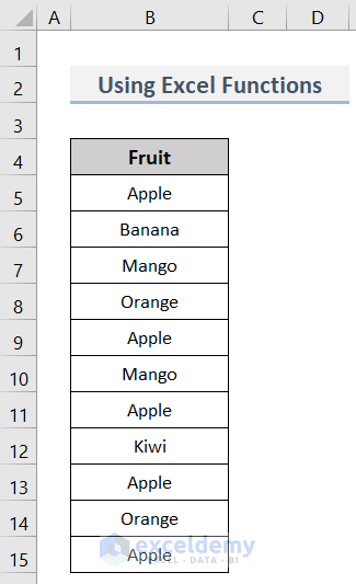
- Paste it into a new worksheet.
- Select the range B5:B15 > go to the Data tab.
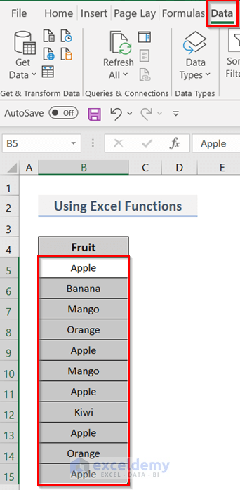
- Data Tools group > Remove Duplicates.
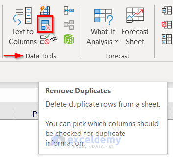
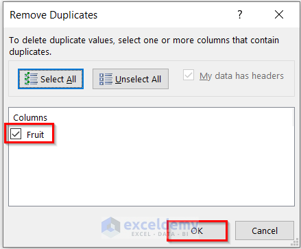
- The Remove Duplicates window will pop up.
- Go to Columns.
- Put a tick mark on the column in which you want to create the unique list.
- Click OK.
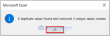
- A message box will appear showing the number of duplicates removed and the number of remaining unique values.
- Click OK.
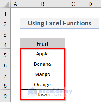
- You will see the unique values only in the Fruit column.
- Select the range (B5:B9) > Formulas tab > Defined Names group > Define Name.
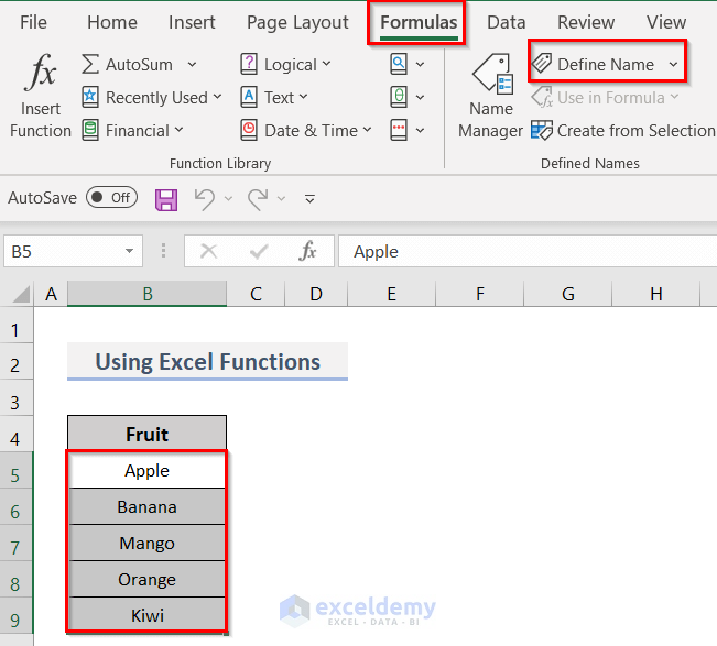
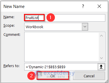
- The New Name window will appear.
- Go to Name > type FruitList > OK.
- Return to the previous or main worksheet and create the dynamic filter search box. We need to create a search box and then link it to a cell.
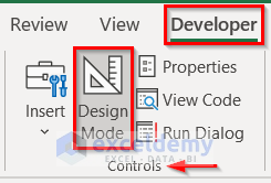
- Go to the Developer tab > Controls group > Insert dropdown > ActiveX Controls > Combo Box.
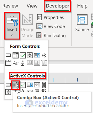
- Click any place in the worksheet and the Combo Box will be inserted.

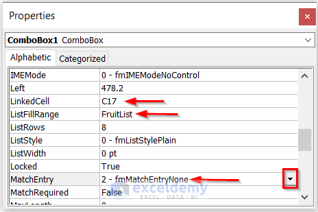
- Select Properties with a right-click on the Combo Box.
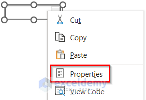
- Properties window > LinkedCell > C17 > ListFillRange > FruitList > MatchEntry dropdown > 2 – fmMatchEntryNone.
- Keep the selection on the Combo Box, go to the Developer tab again > Controls group > click on Design Mode.
- Exit the Design Mode and enter any text in the Combo Box.
- Anything you type will instantly appear in cell C17.
To set the data, connect everything using helper columns. For example, we have used two helper columns H1 & H2. For this, we will use IF, ISNUMBER, SEARCH, and SUM functions in Excel respectively.
- Go to the H1 column and put the serial number (1 to 11) for each record in the dataset.
- Select cell H5 of the H2 column.
- Enter the following formula in the cell (H5) to search for the desired data:
=IF(ISNUMBER(SEARCH($C$17,C5)),G5,"")- Press the Enter key.
- Drag the fill handle to copy the formula up to cell H15.
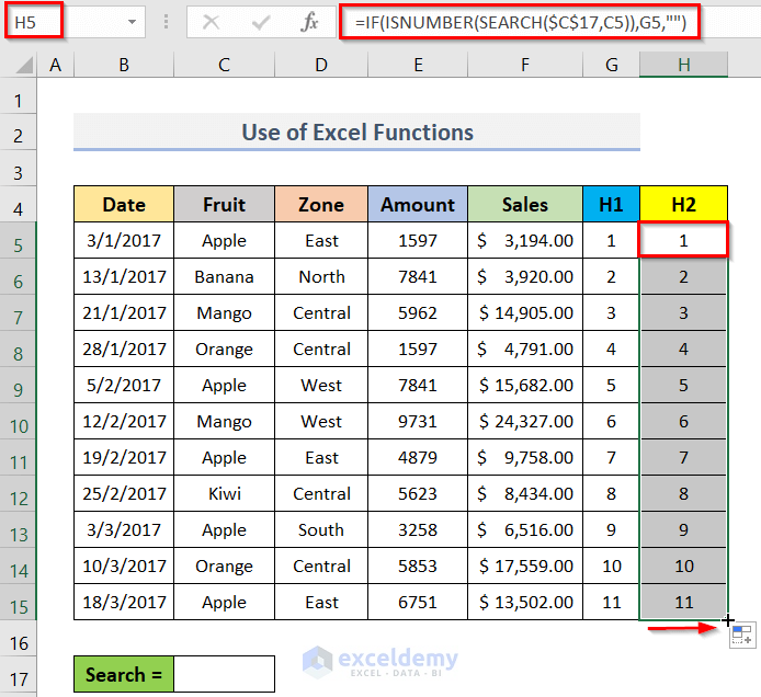
This formula will look for the data in the search box (connected to cell C17) in the cell that contains the fruit’s name. If a match is found, this formula shows the dataset’s row number; otherwise, it displays a blank.
- For example, if you type Apple in the search box, row numbers 1, 5, 7, 9, and 11 contain Apple.
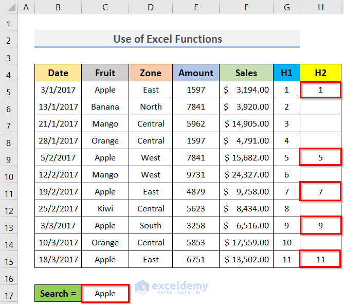
- We created a dynamic filtering search box in Excel.
How to Find Number of Search Matches Using Array Formula in Excel?
We will demonstrate the process for getting the number of matches for any specific data in Excel using an array formula. Let’s say we want the number of matches in the C17 column in the dataset below. The steps to find it are below.
Steps:
- Go to cell C17.
- To get the number of matches, enter the following formula in cell C17:
=SUM(-(ISNUMBER(SEARCH("Apple",$C$5:$C$15))))- Press Ctrl + Shift + Enter to close this array formula.
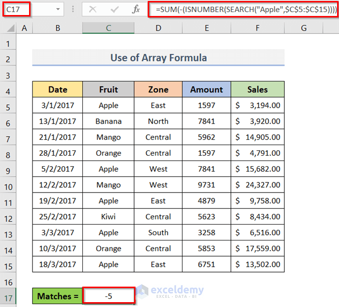
In the formula, the Apple is the desired data we will look for in the C5:C15 range.
- The number of matches for Apple is 5 in cell C17.
Things to Keep in Mind
To create a search box in Excel properly, we must maintain the points below:
- In the Conditional Formatting window, double-check that you entered the formula correctly.
- To verify that there is no deviation, use the $ symbol just like in the formulas above.
- More columns are added to the formula by using the & sign. So, do not finish the formula with the & sign.
Download the Practice Workbook
Download the practice workbook from here.
Related Articles
<< Go Back to Data Management in Excel | Learn Excel
Get FREE Advanced Excel Exercises with Solutions!
