How to Create Search Box in Excel with Conditional Formatting (5 Ways)

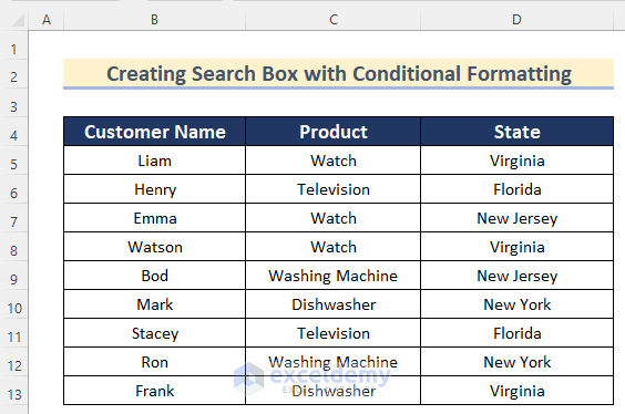
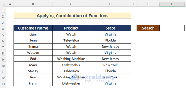
In this article we will demonstrate 5 ways to create a search box in Excel with Conditional Formatting. We’ll use the following dataset containing the Customer Name, Product, and State of a company to illustrate our methods.

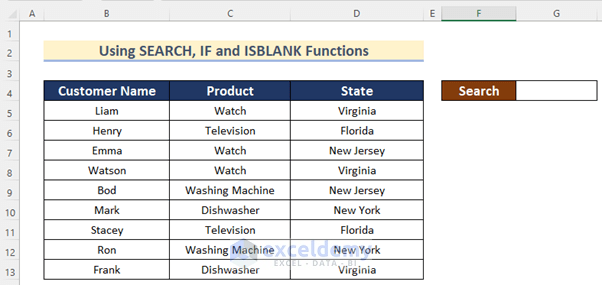
Method 1 – Using the SEARCH, IF, and ISBLANK Functions to Create a Search Box in Excel

In our first method, we’ll use the SEARCH, IF, and ISBLANK functions with Conditional Formatting. The SEARCH function returns a particular string from the given range, and the ISBLANK function is used to check if a cell is empty or not, returning True or False.

Steps:

• Select the range B5:D13.
• Go to the Home tab >> click on Conditional Formatting.

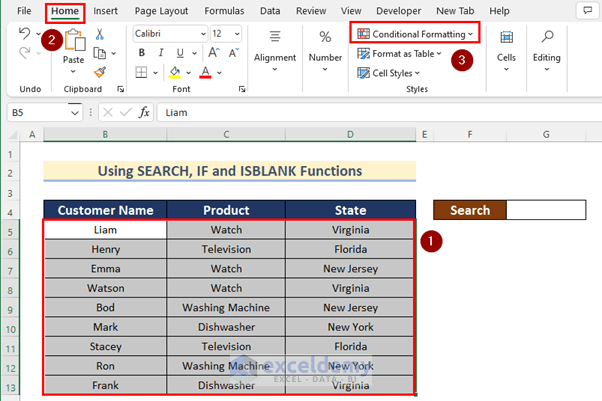
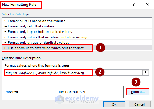
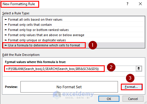
• Select New Rule.

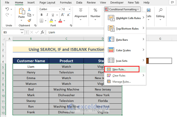
The New Formatting Rule box will open.

• Select Use a formula to determine which cells to format.
• Insert the following formula in the box:

Here, we check if Cell G4 is blank or not using the ISBLANK function. If TRUE, 0 is returned, else the SEARCH function will search for the value of cell G4 and adjacent data in columns B, C and D.

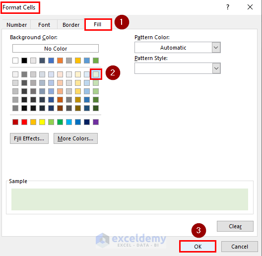
• Click on Format.

The Format Cells box will open.

• Click on the Fill option.
• Select any Background Color of your choice. Here, we select Green, Accent 6, and Lighter 80%.
• Click on OK.

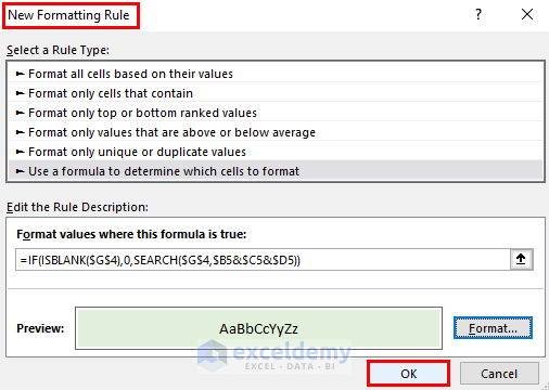
Again, the New Formatting Rule box will appear.

• Click on OK.

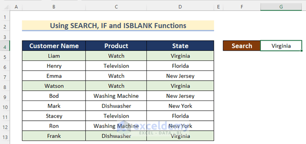
Now, if you enter a value in cell G4 that is in the selected cell range, the matching cell and its corresponding cells will be formatted as specified.

• Insert Virginia in cell G4.

The ranges B5:D5, B8:D8, and B13:D13 will be formatted according to the formula used in Conditional Formatting.

Read More: How to Create a Search Box in Excel

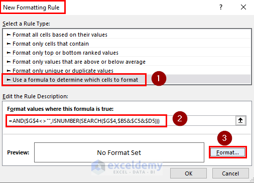
Method 2 – Using a Combination of Functions to Create a Search Box in Excel with Conditional Formatting

We can also create a search box using the AND, ISNUMBER, and SEARCH functions. The ISNUMBER function checks if a cell contains a number or not. The AND function checks multiple arguments and if all the arguments are True then it will return True else False.

Steps:

• Follow the steps shown in Method 1 to open the New Formatting Rule box.
• Select Use a formula to determine which cells to format.
• Insert the following formula in the box:

Here, we check if cell G4 is a number with the ISNUMBER Function. If TRUE, 0 is returned, else the SEARCH function will search for the value of cell G4 and adjacent data in columns B, C and D.

• Click on Format.

• Change the Format where the formula is True by going through the steps shown in Method 1.
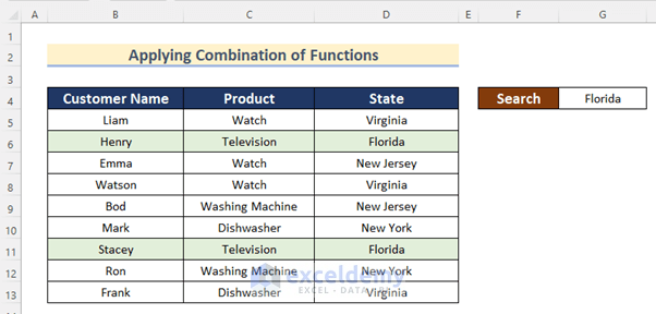
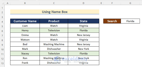
• Insert Florida in cell G4.

The ranges B6:D6 and B11:D11 are formatted according to the formula we used in Conditional Formatting.

Read More: How to Create a Search Box in Excel for Multiple Sheets

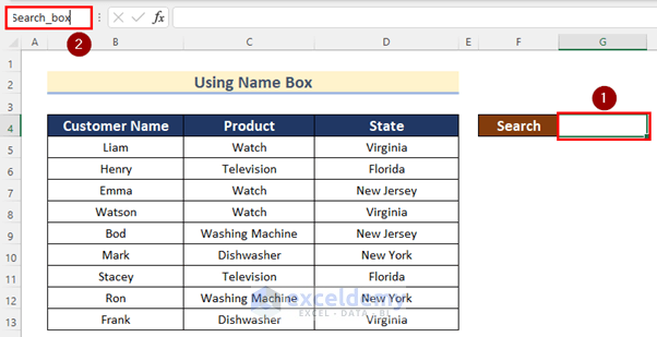
Method 3 – Using a Name Box to Create a Search Box with Conditional Formatting

Now let’s create a search box using a Name Box with Conditional Formatting.

Steps:

• Select cell G4.
• Type Search_box in the Name Box.
• Press ENTER.

• Follow the steps shown in Method 1 to open the New Formatting Rule box.
• Select Use a formula to determine which cells to format.
• Insert the following formula in the box:

• Click on Format.

• Change the Format where the formula is True by going through the steps shown in Method 1.
• Enter Florida in cell G4.

The ranges B6:D6 and B11:D11 are formatted according to the formula we used in Conditional Formatting using the Name Box.

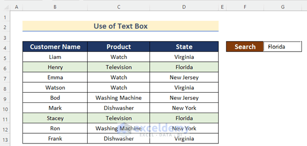
Method 4 – Using a Text Box from ActiveX Controls to Create a Search Box with Conditional Formatting

Steps:

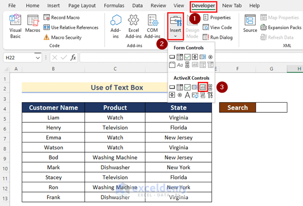
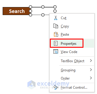
• Go to the Developer tab >> click on Insert >> select Text Box from ActiveX Controls.

• Insert a Text Box and right-click on it.

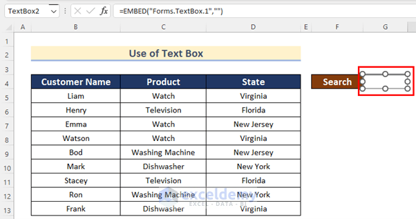
• Click on Properties.

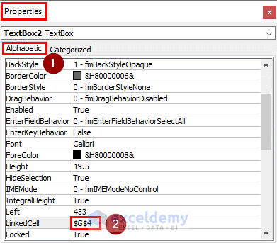
The Properties box will open.

• Select the Alphabetic option.
• Enter cell G4 as the linked cell.

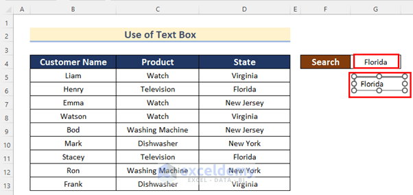
• Enter Florida in cell G4.

This data will automatically be inserted into the Text Box.

• Follow the steps shown in Method 1 to open the New Formatting Rule box.
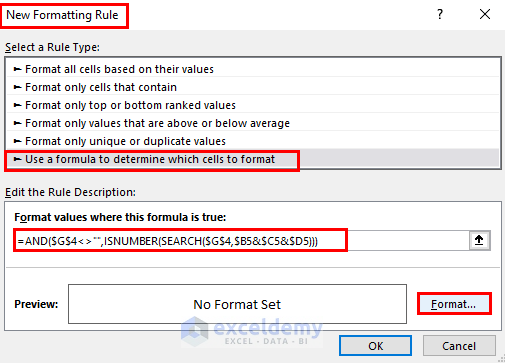
• Select Use a formula to determine which cells to format.
• Insert the following formula in the box:

Here,we check if cell G4 is a number using the ISNUMBER Function. If TRUE, 0 is returned, else the SEARCH function will search for the value of cell G4 and adjacent data in columns B, C and D.

• Click on Format.

The ranges B6:D6 and B11:D11 are formatted according to the formula we used in Conditional Formatting by using a Text Box.

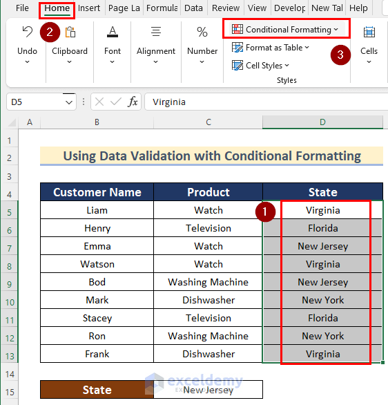
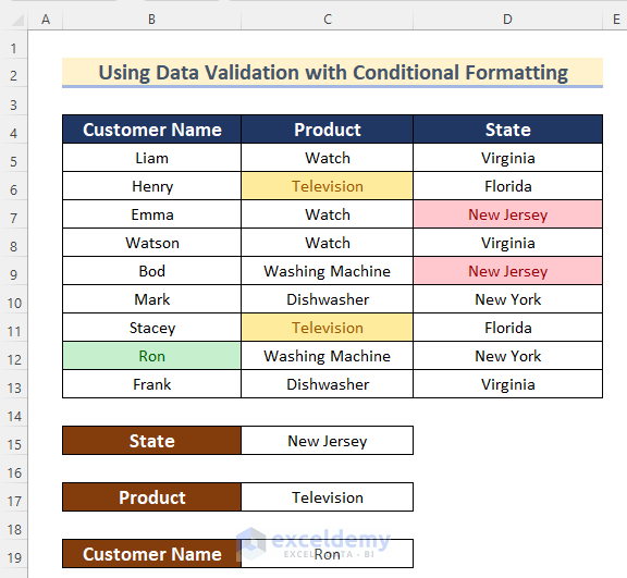
Method 5 – Using Data Validation with Conditional Formatting

In the final method, we will create a search box using Data Validation with Conditional Formatting. We will search for a particular value in a particular column using Data Validation, while preventing input of any data that does not exist in the dataset.

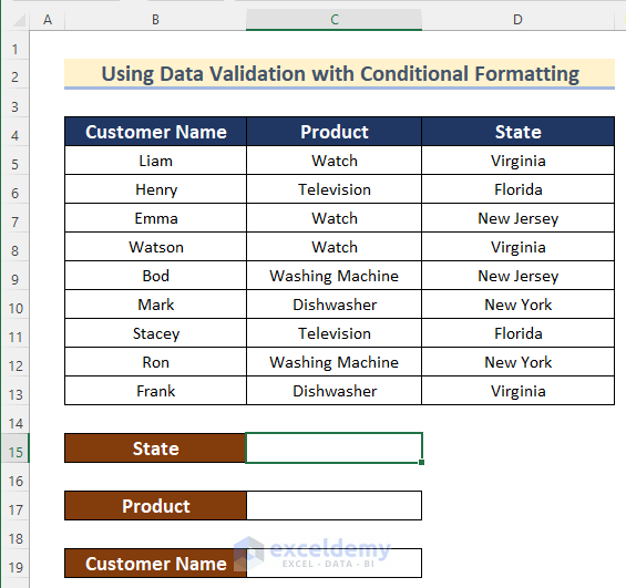
Steps:

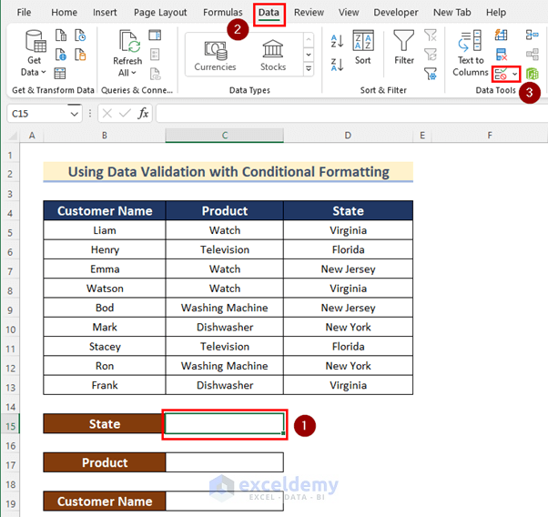
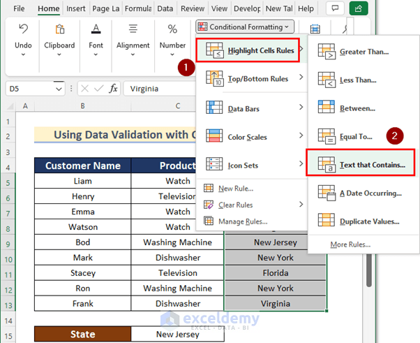
• Select cell C15.
• Go to the Data tab.
• Click on Data Validation.

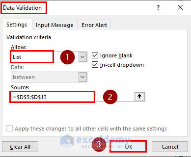
The Data Validation box will appear.

• Select List as the option for Allow.
• Select the range D5:D13 as Source.
• Click on OK.

• Select the Range D5:D13.
• Go to the Home tab.
• Click on Conditional Formatting.

• Click on Highlight Cells Rules >> select Text that Contains.

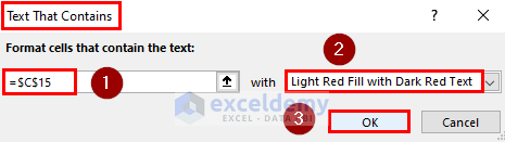
The Text That Contains box will open.

• Select cell C15 in the Format cells that contain the text box.
• Select Light Red Fill with Dark Red Text as Format.
• Click on OK.

• Select New Jersey in cell C15.

The Format will change automatically in cell D7 and cell D9.

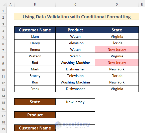
• Similarly, create search boxes for Column B and Column C and format the cells according to your preference using Data Validation with Conditional Formatting.

Download Practice Workbook

Related Articles

• How to Create a Search Box in Excel Without VBA
• Create a Search Box in Excel with VBA
• How to Create a Filtering Search Box for Your Excel Data

<< Go Back to Data Management in Excel | Learn Excel