Download the Free Excel Student Loan Amortization Schedule Template
Feel free to download our free Excel Student Loan Amortization Schedule template. This template will allow you to generate your own personalized student loan amortization schedule.
Click here to enlarge the image
Download Excel Template
Download Excel TemplateFor: Excel 2007 or later
License: Private Use
⏷What Is Student Loan?
⏷Student Loan Amortization Schedule Excel Template
⏵Basic Student Loan Amortization Schedule
⏵Student Loan Amortization Schedule with Extra Payments (Regular/Irregular)
⏵Student Loan Amortization Schedule with Grace Period
⏷Student Loan Amortization Schedule Excel Template Tips
⏷Student Loan FAQs
Understanding Student Loans
A student loan is essentially a loan taken out by students to cover educational expenses such as tuition fees, textbooks, and other related costs. These loans can be obtained from various sources, including federal and state governments or private institutions.
Here are some key points about student loans:
- Loan Duration: Typically, student loans have a fixed term of 10 years.
- Interest Rate: They are usually offered at a fixed interest rate.
- Grace Period: Some loans come with a grace period (usually around 6 months) before repayment begins.
- Subsidized vs. Unsubsidized: Students can apply for both subsidized (interest-free during school) and unsubsidized loans based on their financial situation.
Types of Student Loan Amortization Schedules
- Basic Student Loan Amortization Schedule:
- Provides a simple and straightforward amortization table.
- Focuses on regular payments and their impact on the loan balance.
- Student Loan Amortization Schedule with Extra Payments (Regular/Irregular):
- Allows students to make additional payments beyond the regular ones.
- Helps pay off the loan faster and reduce overall interest.
- Student Loan Amortization Schedule with Grace Period:
- Useful for students who have grace periods within their loan terms.
- Generates an amortization table considering these grace periods.
Read More: Amortization Schedule with Irregular Payments in Excel
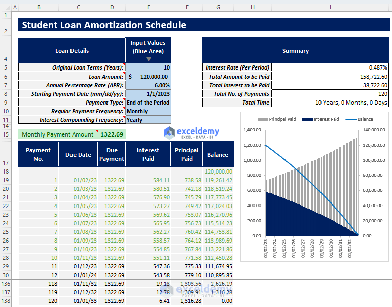
Template 1 – Basic Student Loan Amortization Table
This template takes essential inputs and automatically generates an amortization schedule for your student loan.
Click here to enlarge the image
Here’s how to use it:
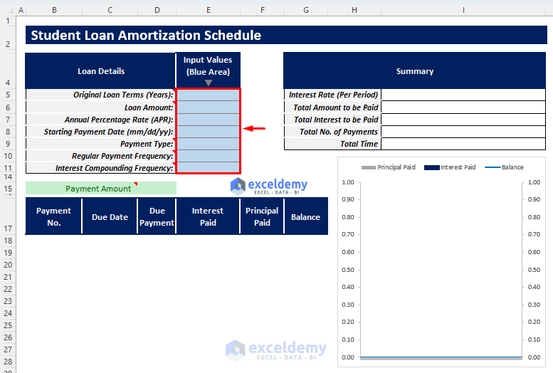
- Input Values:
- In the blue-shaded area, enter the following loan parameters:
- Original Loan Terms (in years)
- Loan Amount
- Annual Percentage Rate (APR)
- Starting Payment Date
- Payment Type (e.g., fixed monthly payments)
- Regular Payment Frequency (e.g., monthly)
- Interest Compounding Frequency (e.g., annually)
- In the blue-shaded area, enter the following loan parameters:
Click here to enlarge the image
- Results:
- The template will calculate your required payment amount and create an amortization schedule.
- You’ll receive an output summary with the following information:
- Interest rate per payment period
- Total amount to be paid over the loan term
- Total interest paid
- Total number of payments
- Total repayment time
- Summary Chart:
- The template also includes a chart showing the trends in interest paid, principal paid, and remaining balance throughout the loan tenure.
Feel free to explore the template and adapt it to your specific loan details. It’s a valuable resource for students managing their educational finances.
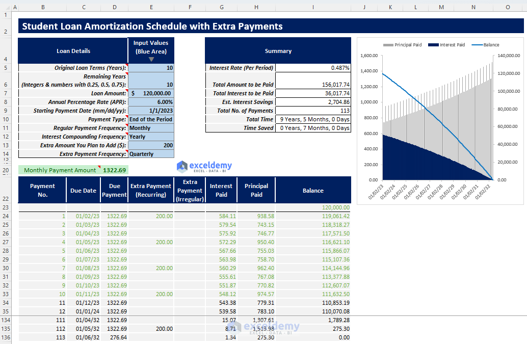
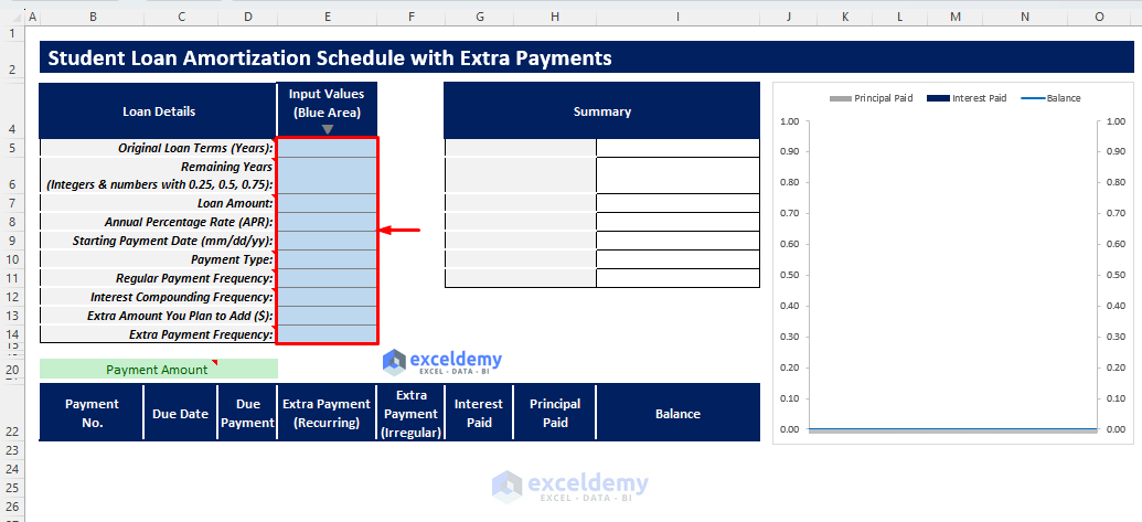
Template 2 – Student Loan Amortization Schedule with Extra Payments (Regular/Irregular)
In this template, you can input the basic necessary details as in the previous template, but you also have the option to add extra regular or irregular payment entries. After inserting the inputs, the template will automatically generate a special amortization schedule and a summary chart. The output summary includes essential information such as estimated interest savings and time saved.
Click here to enlarge the image
Here’s how to use it:
- Input Values:
- In the blue-shaded area of the Input Values column, enter the loan parameters specified in the Loan Details section.
Click here to enlarge the image
-
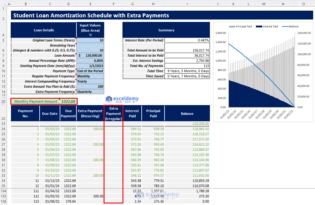
- If you want to make extra irregular payments, add them in the Extra Payments (Irregular) column.
Click here to enlarge the image
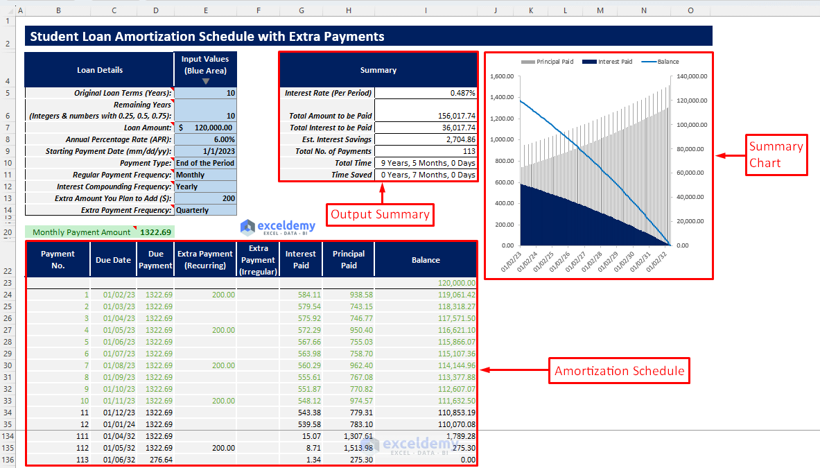
- Results:
- The finalized student loan amortization schedule will be generated based on your inputs.
- You’ll receive an output summary containing:
- Estimated interest savings
- Time saved
- You’ll receive an output summary containing:
- The finalized student loan amortization schedule will be generated based on your inputs.
- Summary Chart:
- Visualize the trends in interest paid, principal paid, and remaining loan balance over the loan term using the summary chart.
Click here to enlarge the image
Read More: Amortization Schedule Excel Template with Extra Payments
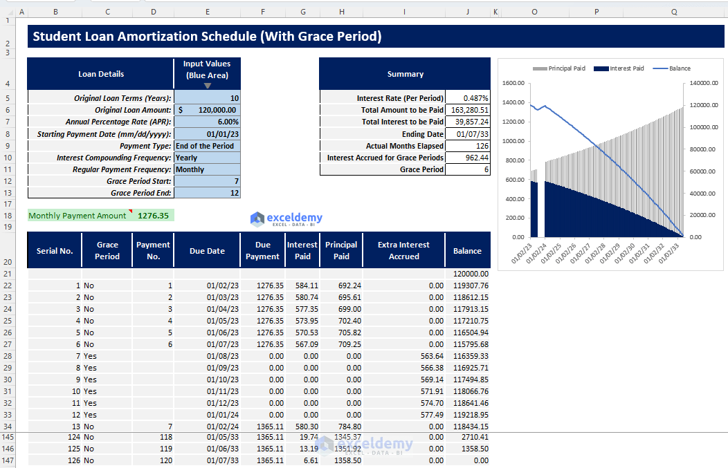
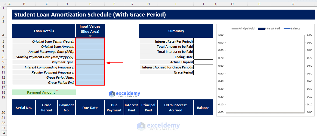
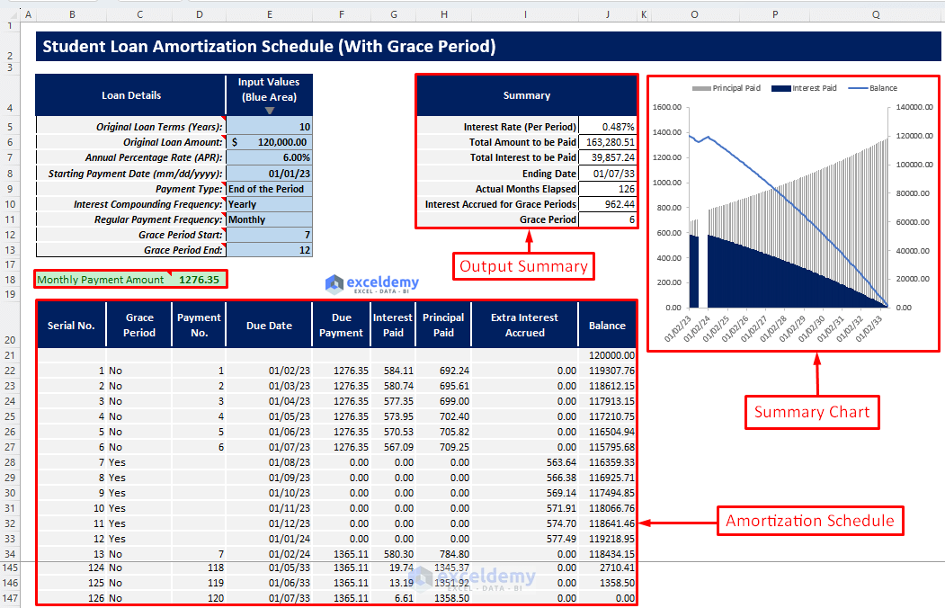
Template 3 – Student Loan Amortization Schedule with Grace Period
This template allows you to utilize the grace period feature for your loan. After inserting the proper inputs and specifying your grace period range, you’ll get a student loan amortization schedule that accounts for the grace period. The output summary and summary chart provide additional insights.
Click here to enlarge the image
Here’s how to use it:
- Go to the Payoff with Grace Period sheet.
- Insert all required inputs, including the Grace Period Start and Grace Period End, in the blue-shaded area of the Input Values column.
Click here to enlarge the image
- The template will calculate your required payment amount, and the output summary will include information such as:
- Interest accrued during grace periods
- Grace period duration
- Actual months elapsed
- Visualize the interest paid, principal paid, and remaining loan balance trend over the loan term using the summary chart.
Click here to enlarge the image
Read More: Multiple Loan Amortization Schedule Excel Template
Student Loan Amortization Schedule Excel Template Tips
- When entering inputs and choosing dropdown options, read the notes provided in the loan parameters to avoid errors.
- Ensure that the interest compounding frequency matches or exceeds your chosen regular monthly payment frequency.
- For extra payment frequency, select a multiple of your regular payment frequency to avoid errors.
Student Loan FAQs
- What Are Subsidized and Unsubsidized Student Loans?
- Subsidized loans are federal loans where students don’t pay interest during school; repayment starts after graduation.
- Unsubsidized loans accrue interest while students are in school.
- Federal vs. Private Loans:
- Federal loans come from the government, often with lower interest rates.
- Private loans are from private institutions or banks and are always unsubsidized.
- Grace Period for Student Loans:
- Grace periods allow borrowers to delay regular payments without penalties.
- Interest may still accrue during grace periods, depending on the loan type.
- Repaying Student Loans with Credit Cards:
- Generally, federal loans can’t be paid with credit cards.
- Private loans may allow credit card payments, but extra charges apply.
Related Articles
- Preparing Bond Amortization Schedule in Excel
- Excel Interest Only Amortization Schedule with Balloon Payment Calculator
- Amortization Schedule with Balloon Payment and Extra Payments in Excel
- ARM Amortization Schedule Excel Template
- Excel Car Loan Amortization Schedule Template
- Excel Car Loan Amortization Schedule with Extra Payments Template
<< Go Back to Amortization Schedule | Finance Template | Excel Templates
Get FREE Advanced Excel Exercises with Solutions!
