We can perform various finance-related tasks in Microsoft Excel very easily. In this article, you will learn about how to prepare a bond amortization schedule in Excel. We will be using the Microsoft 365 version, however, you can follow this article using any Excel version from 2003.
Method 1 – Setting Up Dataset
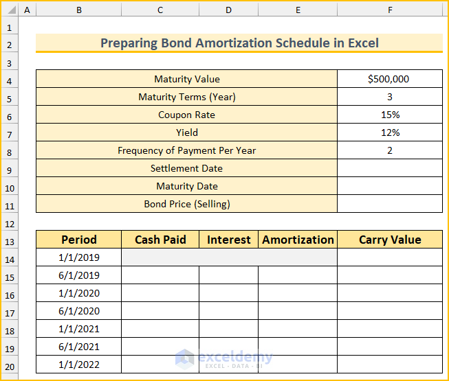
We will input the required values in this step. The bond’s maturity value is $500,000, and its duration is 3 years. The coupon rate and yield are 15% and 12%, respectively. The interest payment is due semi-annually, and the settlement date is January 1, 2019. Use the DATE, YEAR, MONTH, and DAY functions in this step.
- Type the following values.
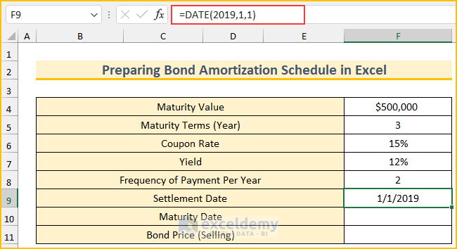
- Type this formula to enter the settlement date. You can type this manually, it is better to input the date using this function.
=DATE(2019,1,1)
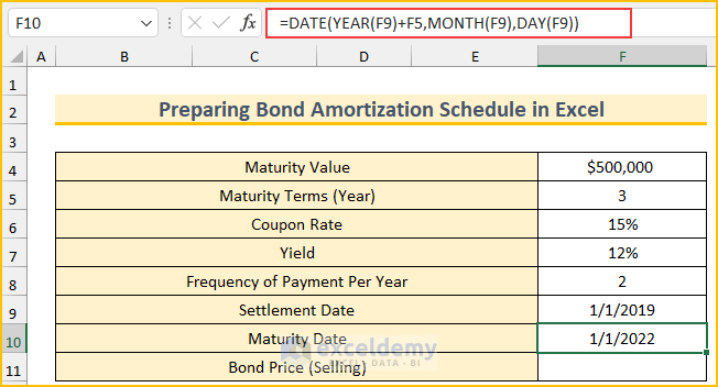
- Type another formula to calculate the maturity date. We are finding the year value from the settlement date and adding the terms. We are keeping the month and day the same as the settlement date.
=DATE(YEAR(F9)+F5,MONTH(F9),DAY(F9))
Method 2 – Creating Bond Amortization Schedule
We will create the amortization schedule using the calculated values from the previous step. Use the PRICE, ABS, and IF functions in this step. The Fill Handle will be used to AutoFill the formulas.
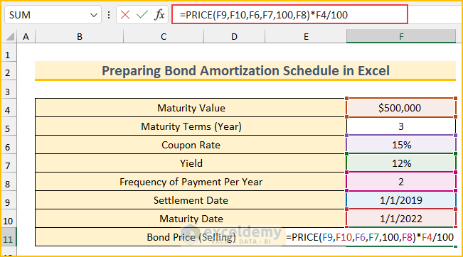
- Type this formula in cell F11 to get the value of the bond price (selling).
=PRICE(F9,F10,F6,F7,100,F8)*F4/100
Formula Breakdown
- PRICE(F9,F10,F6,F7,100,F8)
- Output: 107.376.
- Put 100 inside the PRICE function because by definition this function “returns the price of $100 par value of a bond”. The output from the function is the percentage value.
- The formula reduces to → 107.376*F4/100
- Output: 536879.932.
- We multiplied that value by the maturity value and then divided it by 100 to get the bond price.
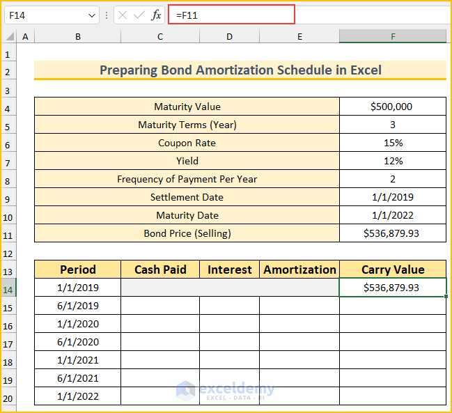
- Type another formula in cell F14.
=F11
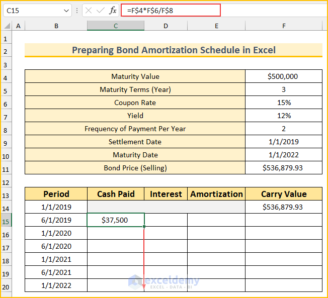
- Type this formula to find the value of cash paid.
=F$4*F$6/F$8
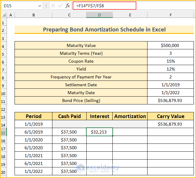
- Type the following formula to calculate the interest amount.
=F14*F$7/F$8
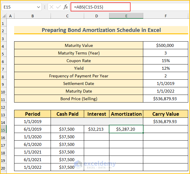
- Type this formula to return the amortization value.
=ABS(C15-D15)
- Type this formula to calculate the carrying value.
=IF(F$4<F$11,F14-E15,F14+E15)
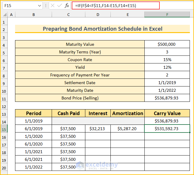
Formula Breakdown
- This is a conditional formula. The condition is that the “maturity value is less than the bond selling price”. When this is true, the F14-E15 will be executed.
- Then, when the condition is false, the F14+E15 will be the output.
- Select the cell range D15:F15 and fill the remaining cells as shown in the following animated image.
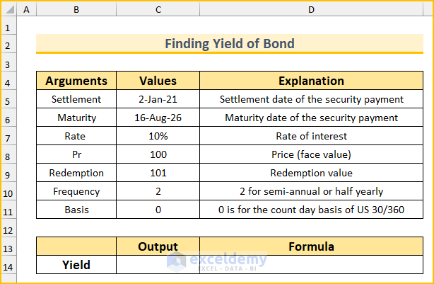
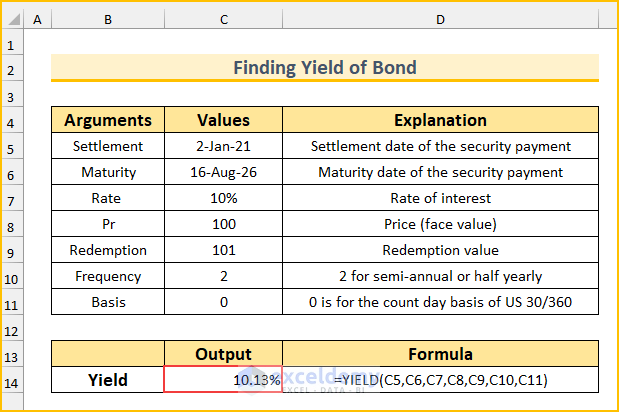
Bond Yield Calculator in Excel
We will use the YIELD function to create a bond yield calculator in Excel. Use the FORMULATEXT function to display the formula. The frequency of payment is semi-annually we used the value 2 for that reason.
Steps:
- Type all the details in the values column. The explanation column is there to clarify the arguments.
- Type this formula in cell C14 to calculate the bond’s yield to maturity.
=YIELD(C5,C6,C7,C8,C9,C10,C11)
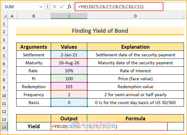
- Press ENTER. Get the yield. Now, you can change the values of the argument and it will return the revised yield.
Download Practice Workbook
You can download the Excel file from the link below.
Related Articles
- Excel Interest Only Amortization Schedule with Balloon Payment Calculator
- Amortization Schedule with Balloon Payment and Extra Payments in Excel
- Multiple Loan Amortization Schedule Excel Template
- Excel Car Loan Amortization Schedule with Extra Payments Template
- Excel Car Loan Amortization Schedule Template
- Excel Student Loan Amortization Schedule
- ARM Amortization Schedule Excel Template
<< Go Back to Amortization Schedule | Finance Template | Excel Templates
Get FREE Advanced Excel Exercises with Solutions!
