Download our free Interest Only Loan Amortization Schedule with Balloon Payment template for Excel to generate your own amortization schedule incorporating interest-only periods and balloon payments.
Click here to enlarge the image
Download Excel Template
Download Excel TemplateFor: Excel 2007 or later
License: Private Use
What Is a Loan Amortization Schedule?
A loan amortization schedule is a loan repayment visualization table. Generally, it shows all the required outputs of a loan repayment procedure such as Due Payment, Due Date, Interest Paid, Principal Paid, Remaining Balance etc. Such a schedule enables easily visualizing what amounts are payable at different periods, and the outstanding amounts required to settle a loan.
What Are Interest Only Periods?
Interest-only periods indicate periods wherein the borrower is approved to pay only the accrued interest without repaying any of the principal.
For example, if a borrower takes a loan of $250,000 for 30 years at a 6% annual interest rate with a 10 year interest only period, only monthly interest payments of $1250 will be due until the 10 years are over. After 10 years, repayment of the principal will begin, along with interest.
What Is a Balloon Payment?
A balloon payment is a payment made by a borrower in a single period to repay the full loan. For example, If a borrower takes a loan for 10 years with a 10 year interest-only period, then only the interest is payable for 10 years, but the whole loan balance will become due as a balloon payment in the next repayment period thereafter.
Read More: Amortization Schedule with Balloon Payment and Extra Payments in Excel
Interest Only Amortization Schedule with Balloon Payment Excel Template
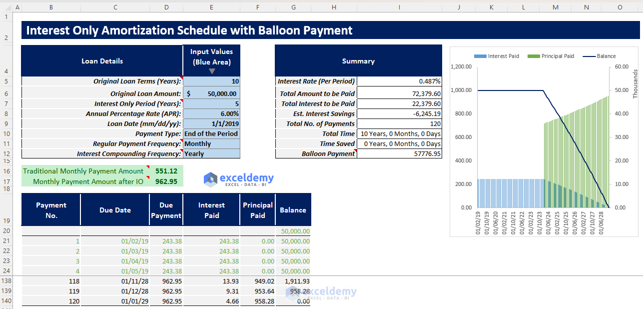
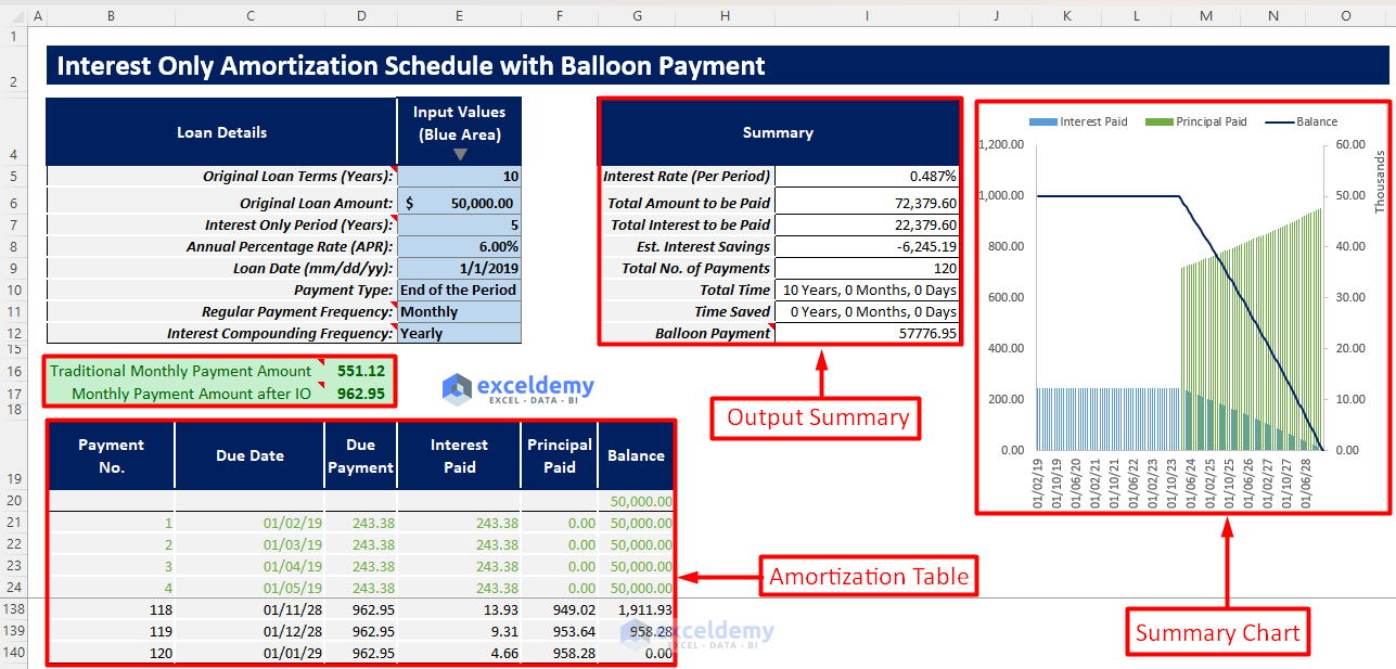
This template takes all your necessary inputs such as loan term, interest-only periods, loan amount, payment frequency, and interest compounding frequency, and generates an amortization table which includes a summary containing balloon payment, total amount to be paid, total interest to be paid, etc. Moreover, it provides a summary chart showing the principal paid, interest paid, and the remaining balance trend during the loan duration.
How to Use This Template
Instructions:
- Open the template and insert all necessary input values in the blue shaded area according to the Loan Details column.
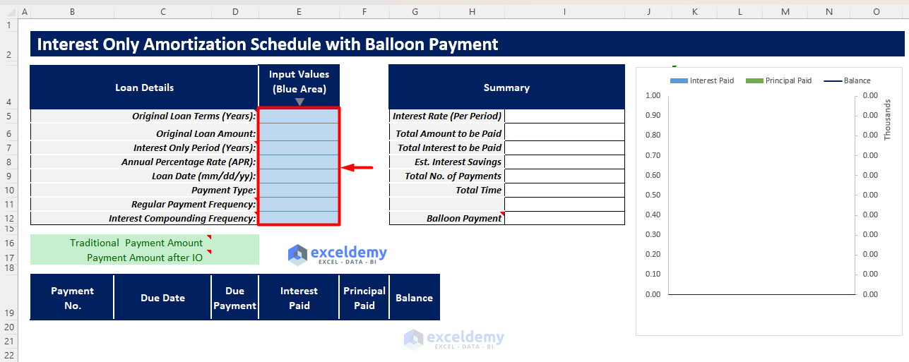
Click here to enlarge the image
- After inserting all the required inputs and selecting all the dropdowns, an amortization table will be generated along with an output summary and a summary chart displaying all the pertinent outputs and balance trends.
- You will also find the EMI if you were not approved for any interest-only period and the required EMI after the interest-only periods in order to pay off the loan within the deadline. Here, if the loan term and interest-only periods are the same, the EMI after interest-only periods will be the whole remaining balance, which is the balloon payment.
Click here to enlarge the image
Read More: Amortization Schedule with Irregular Payments in Excel
Tips for Using the Schedule
- Insert all the inputs properly and refer to the provided notes for instructions.
- When choosing regular payment frequency and interest compounding frequency, the interest compounding frequency must be greater than or equal to the regular payment frequency or you will receive an error.
- In the charts, the dark blue line represents the loan balance trend, the light blue line represents interest paid over the loan term, and the light green line represents the principal paid over the loan term.
Related Articles
- Excel Car Loan Amortization Schedule with Extra Payments Template
- Preparing Bond Amortization Schedule in Excel
- Amortization Schedule Excel Template with Extra Payments
- Multiple Loan Amortization Schedule Excel Template
- Excel Car Loan Amortization Schedule Template
- Excel Student Loan Amortization Schedule
- ARM Amortization Schedule Excel Template
<< Go Back to Amortization Schedule | Finance Template | Excel Templates
Get FREE Advanced Excel Exercises with Solutions!
