What Is an Amortization Schedule in Excel?
An amortization schedule is a table-format repayment plan for monthly bills, loans, or a mortgage. Each payment is subdivided into principal and interest, and the outstanding amount is shown after each payment.
What Are Balloon Payments and Extra Payments?
A balloon payment is a loan form where the monthly payments are lower, with the last payment being significantly larger. Typically used before 2008, the final payment in the system is typically the loan principal while the monthly payments only cover the interest.
Extra payments are one-off payments on the loan to lower the loan amount since it shortens the duration of the loan and thus can reduce the total interest.
Step-By-Step Procedure to Make an Amortization Schedule with Balloon Payment in Excel
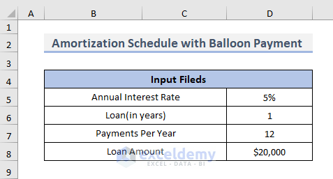
Step 1 – Establish Input Fields
- Define the input cells to make an amortization schedule with a balloon payment.
- Put the Annual Interest Rate, and we’ll use a sample rate of 5%.
- Insert the Loan duration in years, where we’ll put 1.
- Insert the Payments Per Year, which is 12 for a monthly repayment plan.
- Put the Loan Amount (the sample will use $20,000).
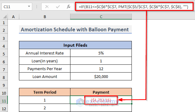
Step 2 – Make a Schedule for the Amortization
- Select the cell where you want to calculate the total payment for the amortization schedule. We selected cell C11.
- Put the following formula into that cell.
=IF(B11<=$C$6*$C$7, PMT($C$5/$C$7, $C$6*$C$7, $C$8), "")- Press Enter to see the result.
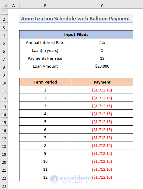
- Drag the Fill Handle down to duplicate the formula over the range or double-click on the Plus (+) symbol.
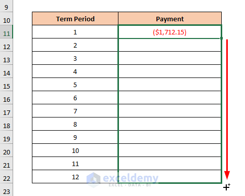
- You will get the payment for each month over the range C11:C22.
How Does the Formula Work?
⇒ PMT($C$5/$C$7, $C$6*$C$7, $C$8): This will return the total period’s payment for a loan.
⇒ IF(B11<=$C$6*$C$7, PMT($C$5/$C$7, $C$6*$C$7, $C$8), “”): This will first compare whether the period is under the loan year or not and then similarly returns the periodic payment.
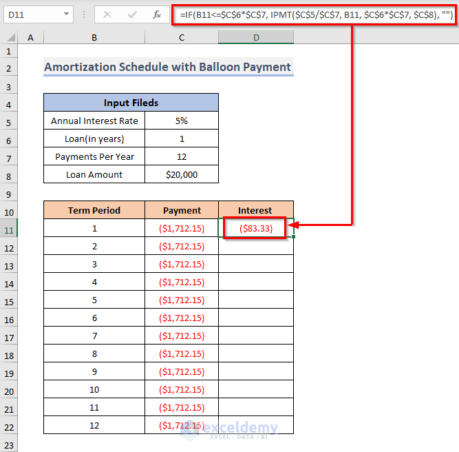
Using the IPMT Function to Calculate the Interest
- Select cell D11.
- Enter the following formula.
=IF(B11<=$C$6*$C$7, IPMT($C$5/$C$7, B11, $C$6*$C$7, $C$8), "")- Hit Enter.
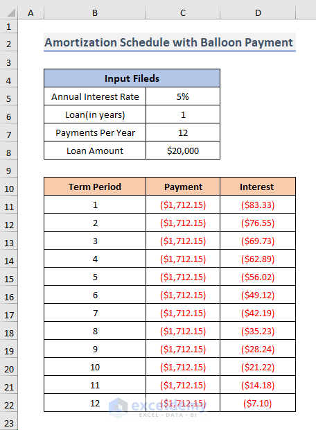
- Drag the Fill Handle down or double-click on the Plus (+) icon.
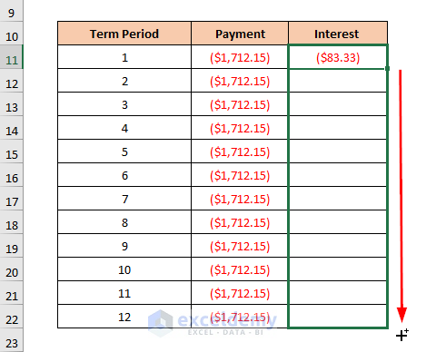
- Here’s the result, showcasing the interest paid in each payment.
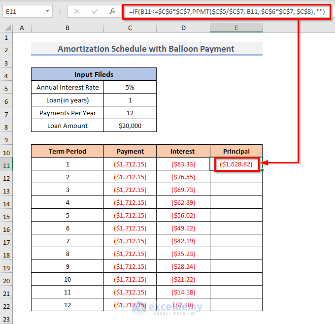
Calculate the Principal Amount Using the PPMT Function:
- Select cell E11 and insert this formula.
=IF(B11<=$C$6*$C$7,PPMT($C$5/$C$7, B11, $C$6*$C$7, $C$8), "")- Press Enter.
- Drag the Fill Handle down or double-click on the Plus (+) symbol.
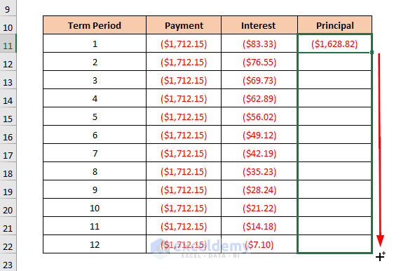
- We can see the principal amounts in cells E11:E22.
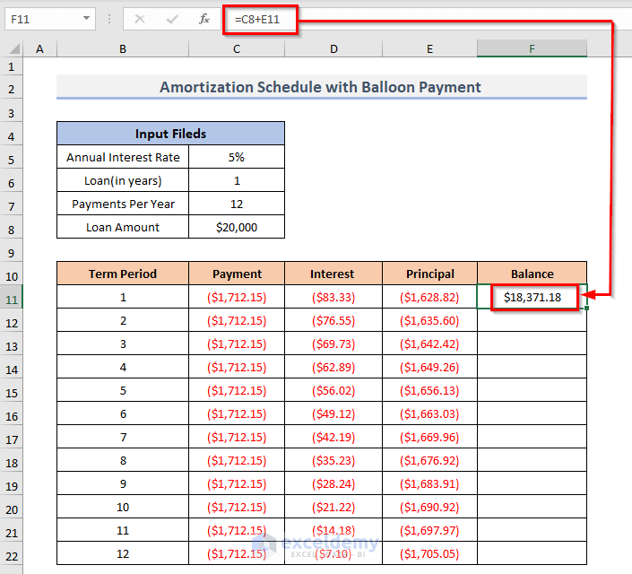
Compute the Remaining Balance
- Select cell F5.
- Put this formula into the cell.
=C8+E11- Press the Enter key to see the result in that cell.
- Select cell F12 and put the following formula there.
=IF(B12<=$C$6*$C$7, F11+E12, "")- Press Enter on your keyboard.
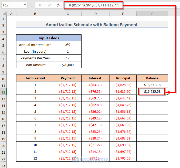
- Drag the Fill Handle down to repeat the formula across the range or double-click on the Plus (+) sign to AutoFill the range.
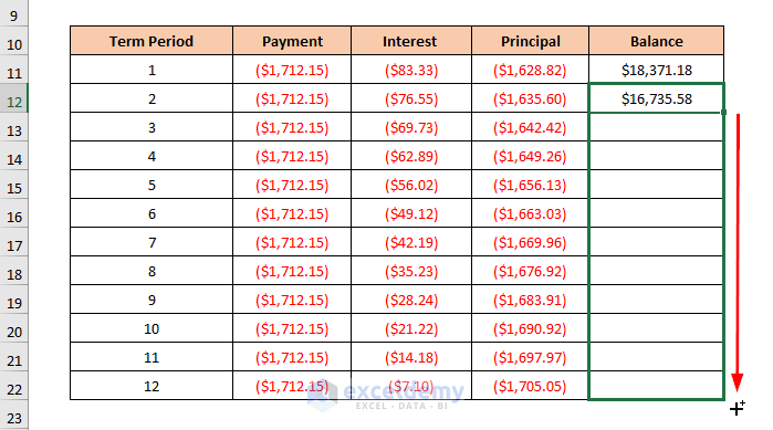
- This will calculate the remaining balance for each period.
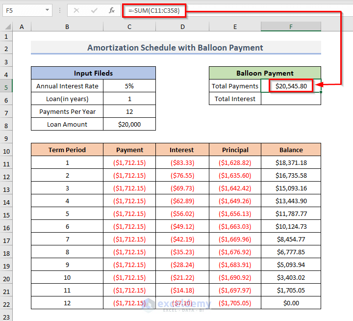
Step 3 – Make a Summary of the Balloon Payment/Loan
- Select the cell to compute the Total Payments for the loan. We selected cell F5.
- Insert the following formula.
=-SUM(C11:C358)- Press Enter to see the result.
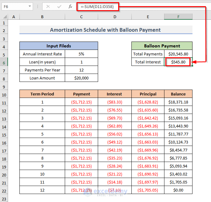
- Select cell F6 and put in the formula for computing the total interest:
=-SUM(D11:D358)- Hit Enter.
Read More: Excel Interest Only Amortization Schedule with Balloon Payment Calculator
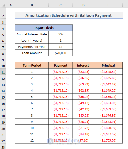
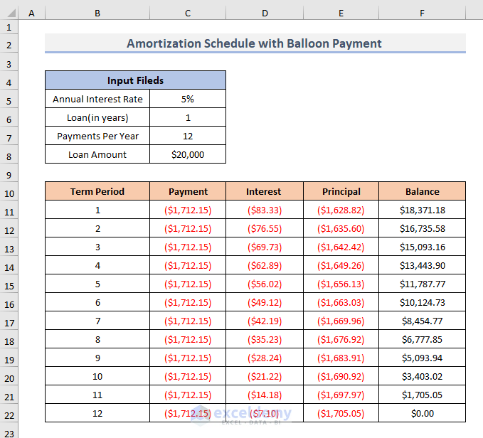
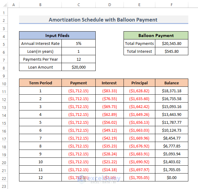
Final Template
This is the final template for the amortization schedule with a balloon payment. You can use the template and change the input cells as per your requirements.
Read More: Multiple Loan Amortization Schedule Excel Template
Step-By-Step Procedure to Make an Amortization Schedule with Extra Payments in Excel
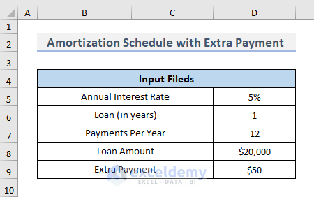
Step 1 – Specify Input Fields
- Put the Annual Interest Rate, and we’ll use a sample rate of 5%.
- Insert the Loan duration in years, where we’ll put 1.
- Insert the Payments Per Year, which is 12 for a monthly repayment plan.
- Put the Loan Amount (the sample will use $20,000).
- Finally, the Extra Payment is $50. We’ll consider a simple example of extra payments every pay period.
- We named each cell with its own named range (removing spaces) to make the template easier the read.
Step 2 – Construct an Amortization Schedule
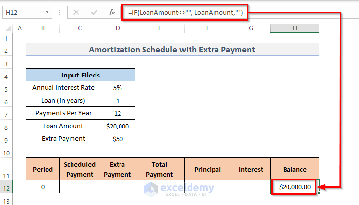
- Select cell H12.
- Enter the following formula into that cell.
=IF(LoanAmount<>"", LoanAmount,"")- Press Enter.
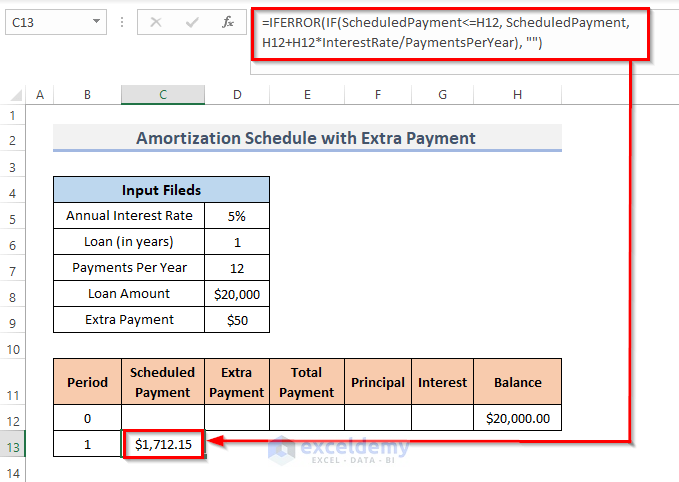
Compute the Schedule Payment
- Select cell C13 and input the following formula.
=IFERROR(IF(ScheduledPayment<=H12, ScheduledPayment, H12+H12*InterestRate/PaymentsPerYear), "")- Hit Enter.
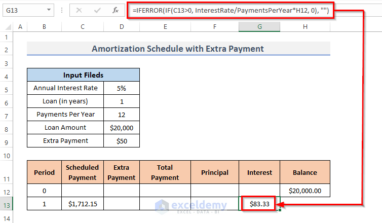
Evaluate the Interest
- Select cell G13 and insert the following formula.
=IFERROR(IF(C13>0, InterestRate/PaymentsPerYear*H12, 0), "")- Hit Enter.
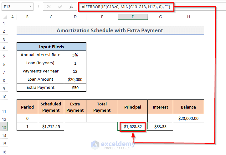
Find the Principal Amount
- Choose cell F13 and put the following formula into it.
=IFERROR(IF(C13>0, MIN(C13-G13, H12), 0), "")- Press Enter.
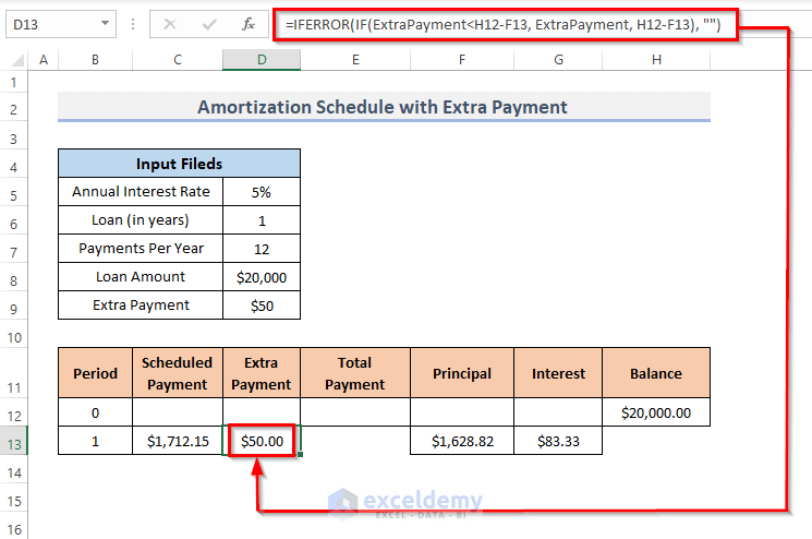
Calculate the Extra Payment
- Select cell D13.
- Put the following formula into that chosen cell.
=IFERROR(IF(ExtraPayment<H12-F13, ExtraPayment, H12-F13), "")- Press Enter.
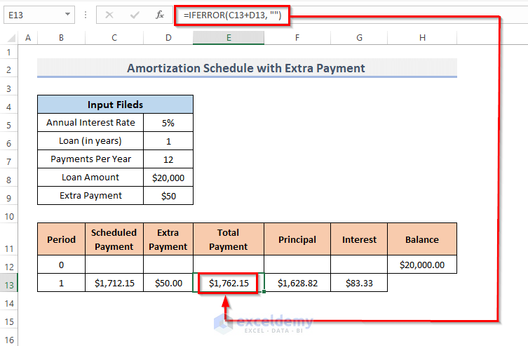
Compute the Total Payment
- Select cell E13.
- Enter this formula into the cell.
=IFERROR(C13+D13, "")- Press the Enter key.
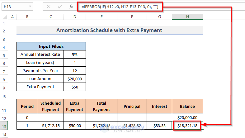
Calculate the Remaining Balance for Each Payment Period
- Select the first next cell for the remaining balance, H13.
- Insert the following formula.
=IFERROR(IF(H12 >0, H12-F13-D13, 0), "")
- Press Enter.
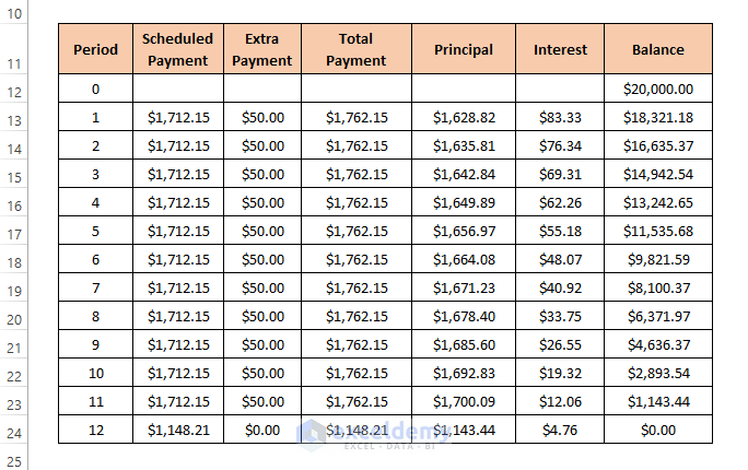
Amortization Schedule
- Repeat the steps for every cell in the table.
This may take a long time. We provided the download files that you can use as ready-made templates.
Read More: Amortization Schedule with Irregular Payments in Excel
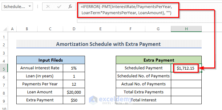
Step 3 – Make a Summary of Extra Payments
- Select the cell for computing the Schedule Payment, H5.
- Insert the following formula:
=IFERROR(-PMT(InterestRate/PaymentsPerYear, LoanTerm*PaymentsPerYear, LoanAmount), "")- Hit Enter.
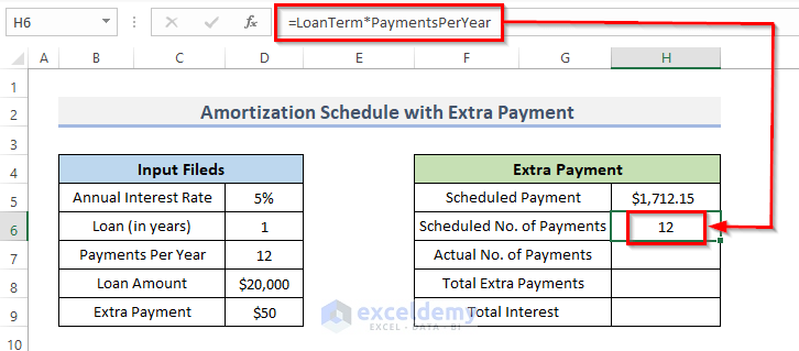
- To compute the Schedule Number of Payment, select cell H6 and insert the following formula.
=LoanTerm*PaymentsPerYear- Hit Enter.
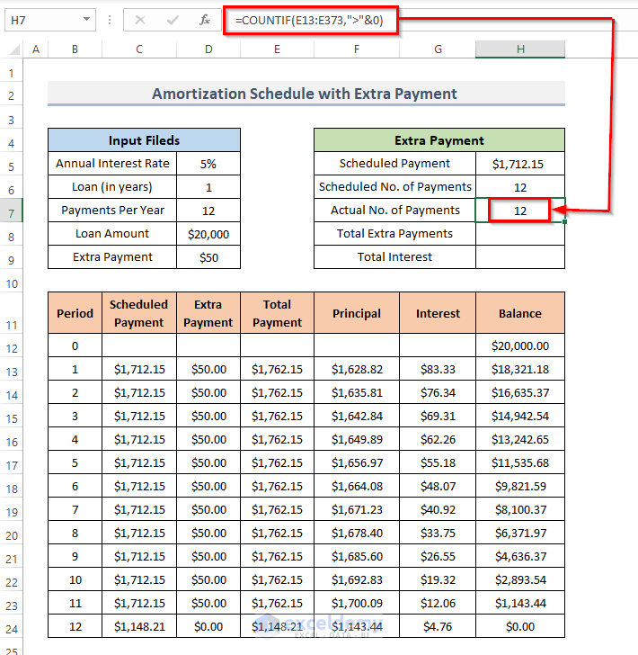
- For the Actual Number of Payments, choose cell H7 and put this formula:
=COUNTIF(E13:E373,">"&0)- Hit Enter.
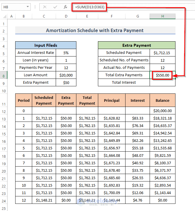
- For Total Extra Payments, select cell H8 and insert the formula there:
=SUM(D13:D363)- Hit the Enter key.
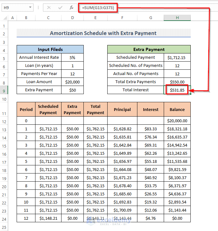
- Calculate the Total Interest in cell H9 with the following formula:
=SUM(G13:G373)- Press Enter.
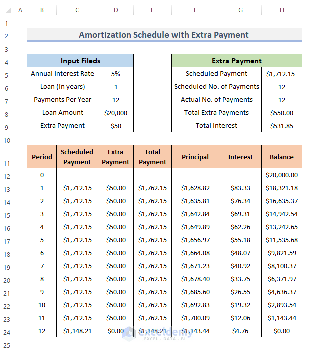
Final Template
Here’s the finalized template you can use.
Read More: Amortization Schedule Excel Template with Extra Payments
Download the Template
Related Articles
- Preparing Bond Amortization Schedule in Excel
- Excel Car Loan Amortization Schedule with Extra Payments Template
- Excel Car Loan Amortization Schedule Template
- Excel Student Loan Amortization Schedule
- ARM Amortization Schedule Excel Template
<< Go Back to Amortization Schedule | Finance Template | Excel Templates
Get FREE Advanced Excel Exercises with Solutions!

There is no ballon in this tool. A ballon payment will have a remaining balance much larger than zero! This is just a loan payment calculator.