This is an overview:
Click here to enlarge the image
Download Excel Template
Download Excel TemplateFor: Excel 2007 or later
License: Private Use
Read More: Excel Car Loan Amortization Schedule Template
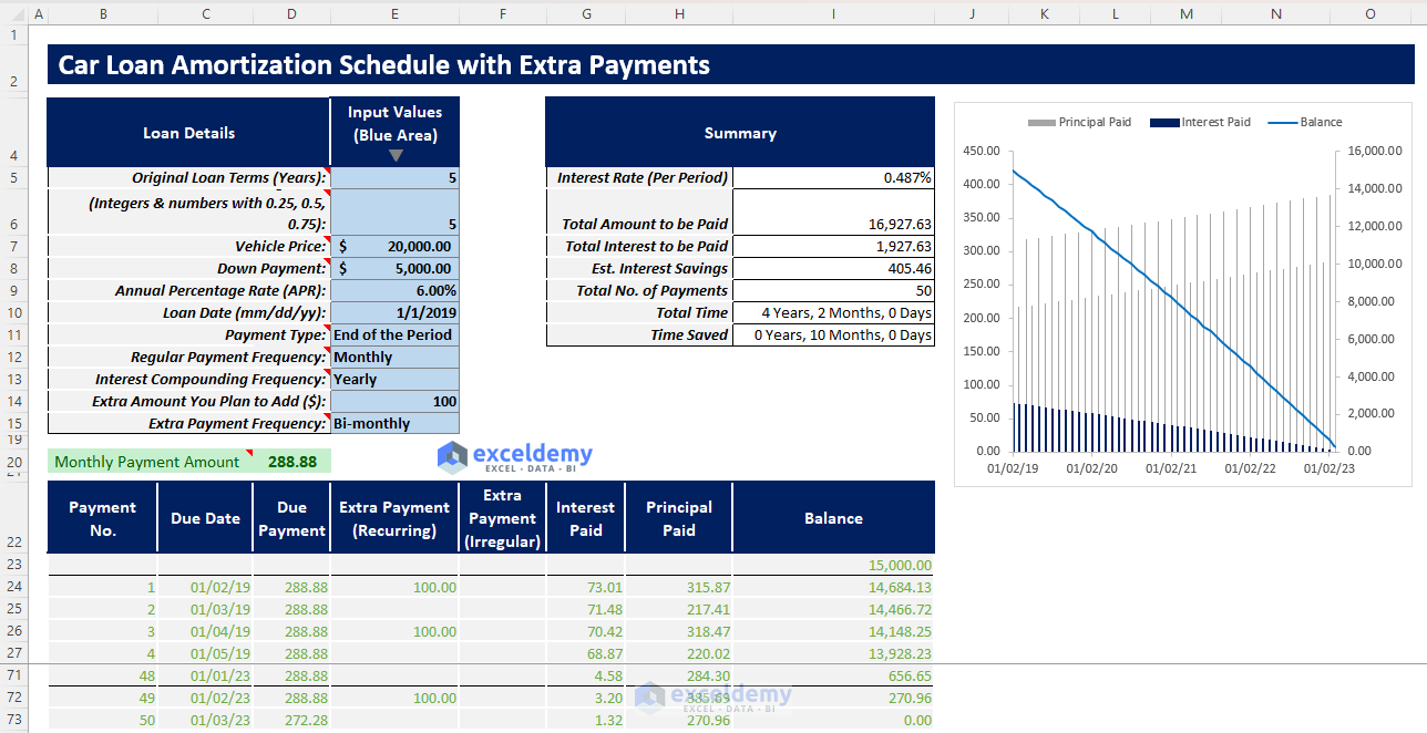
Excel Car Loan Amortization Schedule with Extra Payments Template
How to Use This Template
Instructions:
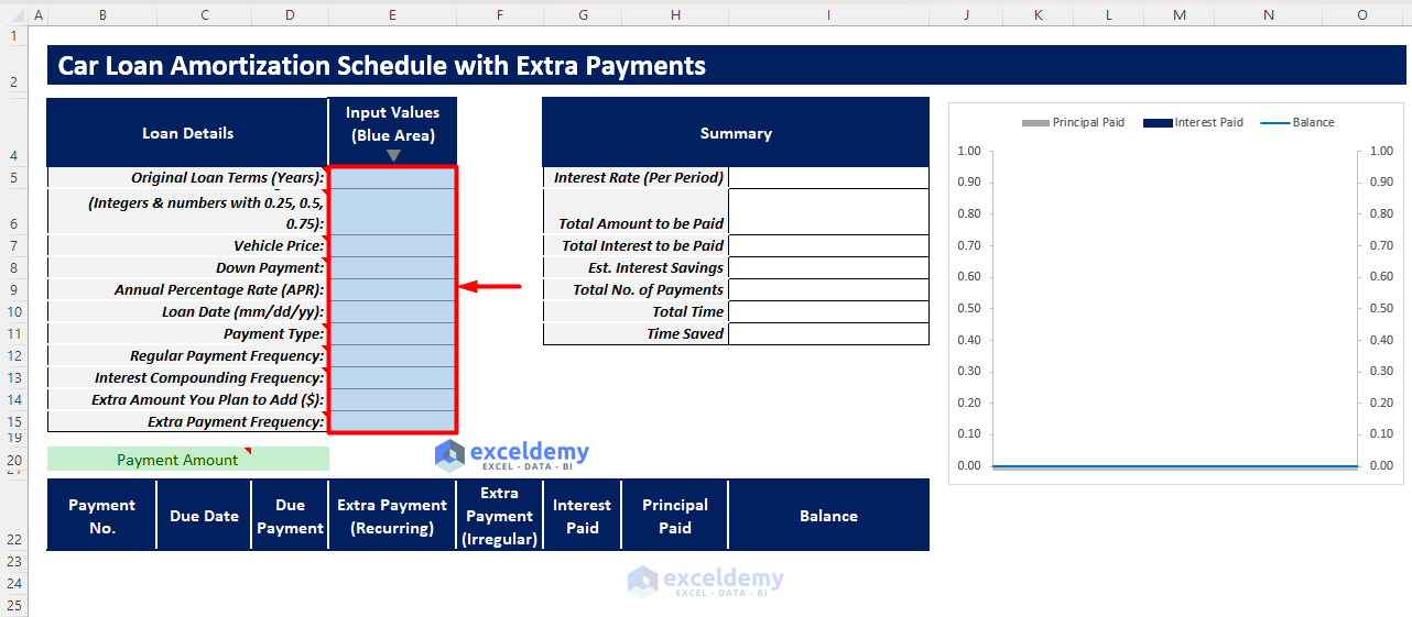
- Open the template and insert your inputs in the blue shaded area.
Click here to enlarge the image
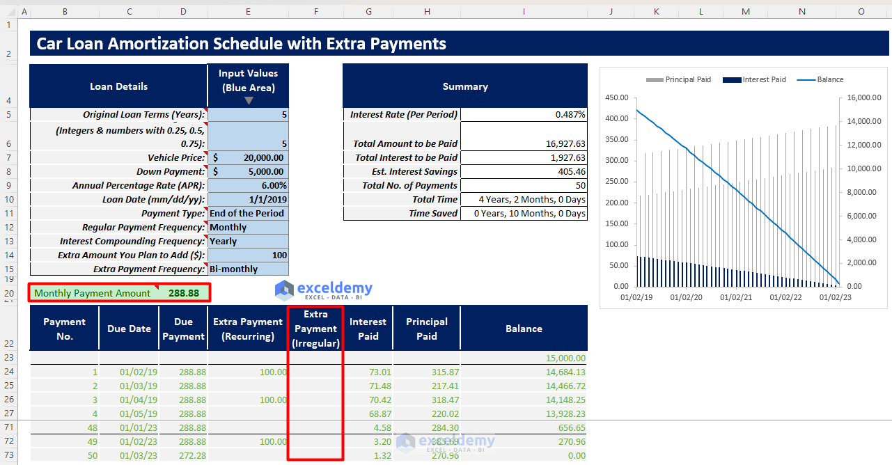
You will get your regular payment amount.
- If you want to make extra irregular payments, enter your data in the Extra Payments (Irregular) column.
Click here to enlarge the image
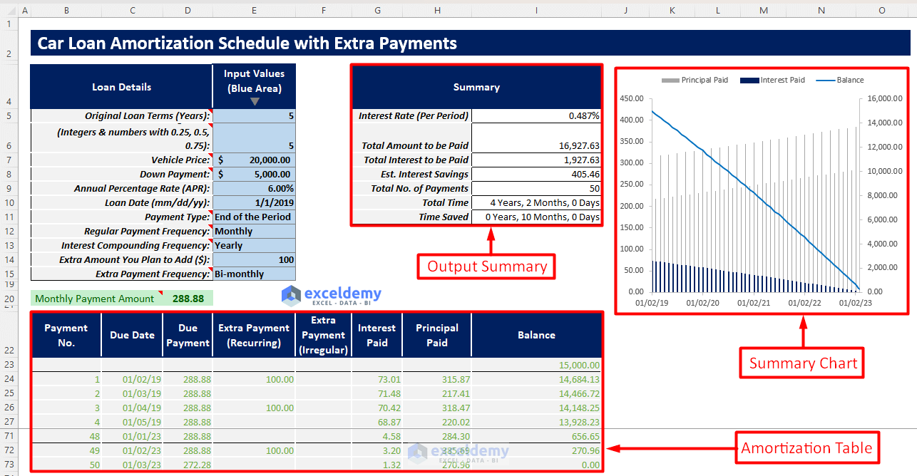
You will get an amortization schedule and an output summary. You will also get a summary chart to visualize balance trends.
Click here to enlarge the image
Read More: Amortization Schedule Excel Template with Extra Payments
Car Loan Amortization Schedule with Extra Payments Tips
- You have to choose interest compounding frequency as equal to or greater than regular payment frequency. Otherwise, it will return an error.
- You have to choose the extra payment frequency as a multiple of the regular payment frequency. Otherwise, the dates won’t match and an error might occur.
Related Articles
- Preparing Bond Amortization Schedule in Excel
- Interest Only Amortization Schedule with Balloon Payment Template Excel
- Amortization Schedule with Balloon Payment and Extra Payments in Excel
- Multiple Loan Amortization Schedule Excel Template
- Excel Student Loan Amortization Schedule
- ARM Amortization Schedule Excel Template
- Amortization Schedule with Irregular Payments in Excel
<< Go Back to Amortization Schedule | Finance Template | Excel Templates
Get FREE Advanced Excel Exercises with Solutions!

Your formula above does not apply the extra payment to the balance. How would I change the formula to account for that extra payment being applied?
Hi MICHELLE,
Greetings and thank you for your inquiry.
To apply the above formula to the extra payment, you need to change the formula in cell H12 as follows:
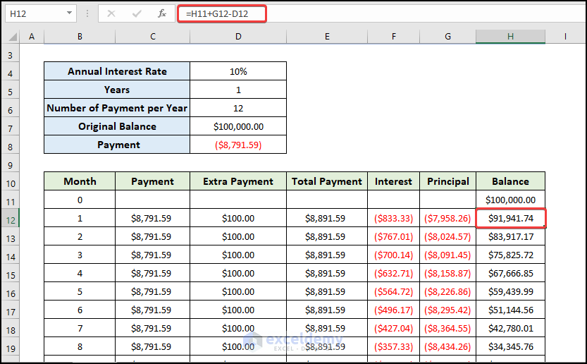
=H11+G12-D12
This means (Original Balance-Principal-Extra Payment).