Most likely you see a checkbox that is mainly used for selecting or deselecting any option. Though the process of adding a checkbox in Excel is quite easy, you may accomplish many creative and dynamic tasks using a checkbox. In this guiding session, I’ll show you all worthy issues including the process of how to add a checkbox in Excel with proper explanation.
How to Add a Checkbox in Excel: 2 Steps
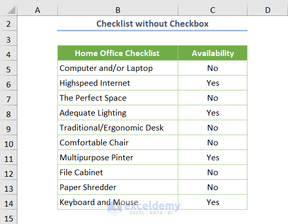
Let’s have a look at the following screenshot where Home Office Checklist is provided along with some open-ended answers e.g. Yes, No. The problem with such a type of answer is that you cannot accomplish various attractive tasks. But Excel provides some outstanding features with the checkbox that will surprise you.
Before exploring the examples, let’s see the process of inserting a checkbox in Excel.
Step 01: Adding Developer Tab
Firstly, look closely at your Excel ribbon and find the Developer tab. If you have the tab, just move to Step 2.
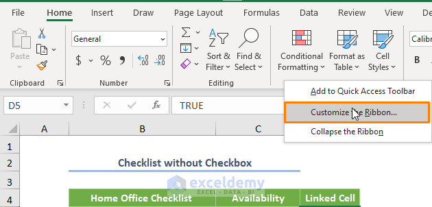
However, if you don’t have the tab, just right-click over any space inside the ribbon and you’ll see some options as shown in the following image. And choose the Customize the Ribbon option.
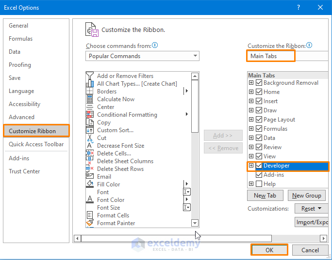
Then, you’ll get the following dialog box namely Excel Options. Therefore check the box before the Developer tab from the Main Tabs. Finally, press OK.
Now, go to the Developer tab and click on the Insert option. Then, choose the Check Box from the Form Controls.
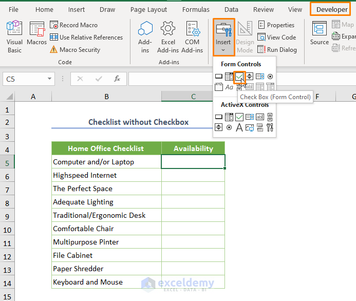
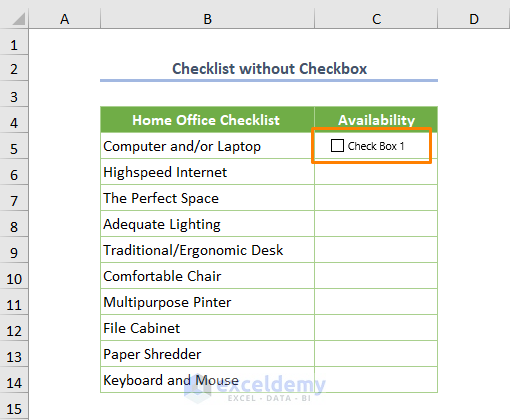
Later, draw a checkbox as illustrated in the following image (in the C5 cell).
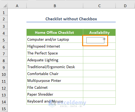
If you stop drawing, you’ll get a box namely Check Box 1(default name).
Thus you may easily add a checkbox in Excel.
Note: Here I showed you the process of adding a checkbox in Excel using the Developer tab. You may visit if you want to add a checkbox without developer tab.
Add Multiple Checkboxes in Excel
Often you might need multiple checkboxes and you have probably three popular ways.
- Firstly, use the shortcut key CTRL + C for copying the checkbox and CTRL + V for pasting that.
- Secondly, you can do that in a single command i.e. CTRL + D. Obviously, you have to select the checkbox by right-clicking before utilizing the above two methods.
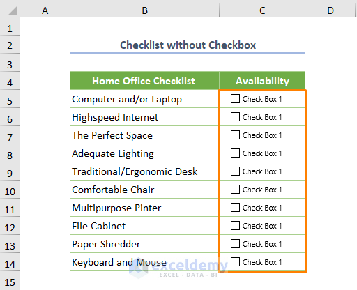
- The last method is quite handy for larger datasets. Just drag down the plus sign of the cell where the checkbox is located (same as the Fill Handle Tool).
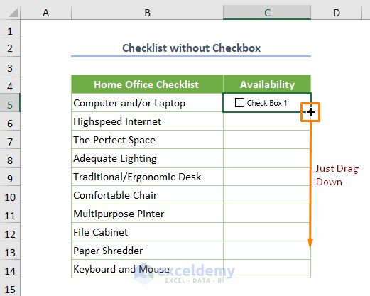
Immediately, you’ll get multiple checkboxes.
Some Basic Edits in a Checkbox
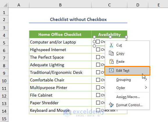
1. Add and Edit the Name of a Checkbox
For specifying the use of the checkbox, you may need to change the default name. The common two methods are-
- Just right-click on the checkbox and choose the Edit Text option from the Context Menu as shown in the following image.
- Firstly right-click on the checkbox and then left-click on the default name. Now, you are able to delete or change the name.
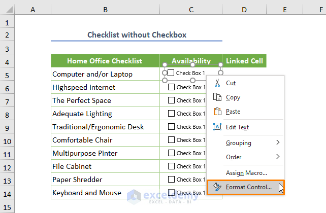
2. Add a Link to a Cell with a Checkbox in Excel
Linking a cell with the checkbox is probably the amazing feature of a checkbox. Because you cannot accomplish analysis unless you link the checkbox with a cell. To do this, initially right-click over the checkbox and choose the Format Control option from the Context Menu.
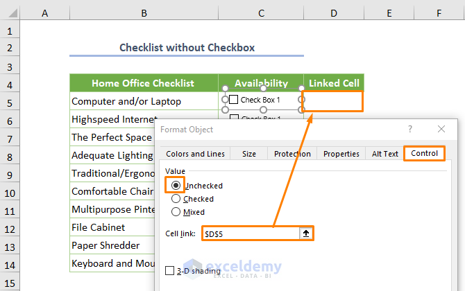
Now, type or select the cell ($D$5) in the space of the Cell Link option from the Control tab where you want to make a link with the checkbox.
Here, you should focus on some key things.
⧬ As the checkbox in the C5 cell where it is unchecked, that’s why it shows the Unchecked value by default. Similarly, it will show the Checked value if the checkbox is checked.
⧬ Alternatively, you might utilize the Mixed option from Value.
⧬ More importantly, the default value of Checked is TRUE and FALSE is for the Unchecked box.
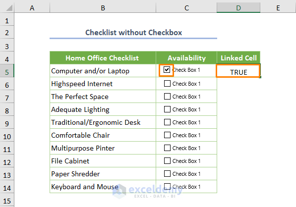
Now, the D5 cell is linked with the checkbox located at the C5 cell. For example, if you check the box, you’ll see TRUE in the D5 cell shortly.
Read More: How to Link Multiple Checkboxes in Excel
Examples of Using a Checkbox in Excel
In this section, you’ll see 4 notable uses of checkboxes in Excel. Let’s understand the uses with the explanation.
1. Add a Checkbox to Create a Simple Checklist
If you understand the process of adding a checkbox and multiple checkboxes, it’s easy for you to create a checklist instead of using open-ended answers.
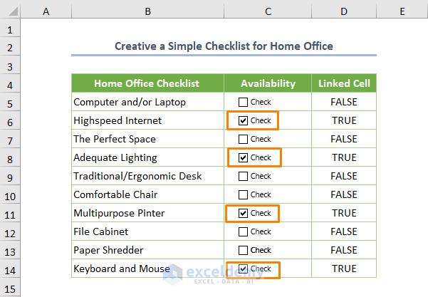
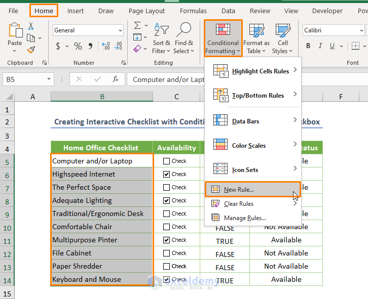
2. Creating an Interactive Checklist Using Conditional Formatting and IF Function
To make the simple checklist interactive, you may use the Conditional Formatting tool. Initially, select the cells (B5:B14) where you want to apply the tool. Then choose the New Rule option from the Conditional Formatting tool which is located in the Styles ribbon of the Home tab.
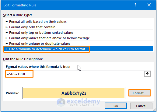
Immediately, you’ll see the following dialog box namely New Formatting Rule, and choose the option Use a formula to determine which cells to format as a Rule Type. Eventually, insert the following formula under the space of Format values where this formula is true.
=$D5=TRUE
Here, D5 is the starting cell of the Linked Cell (linked with the checkbox).
However, click on the Format option from the lower-right corner of the dialog box.
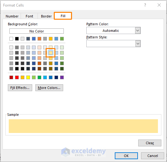
Therefore, make the Font Style as Bold and choose any color.
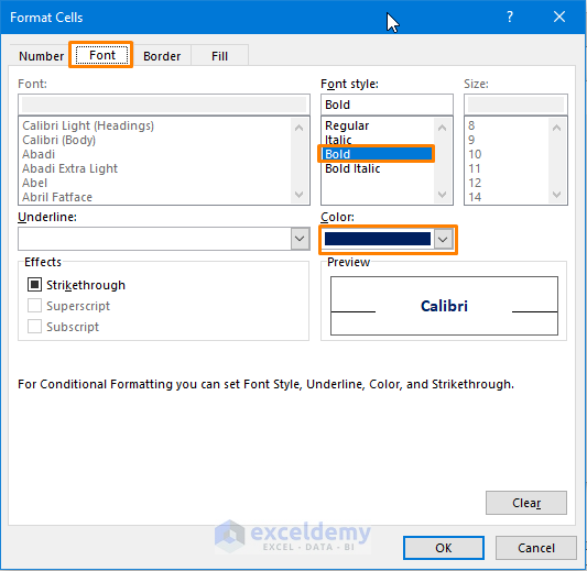
Again, move the cursor over the Fill option and choose a color that you want to use in highlighting.
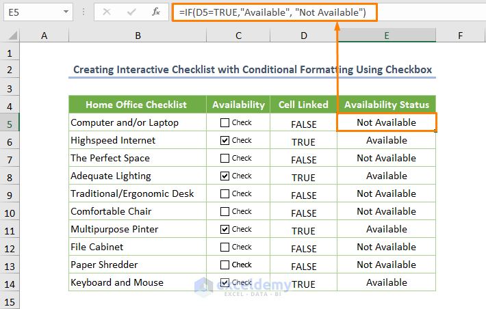
In addition, you may utilize the IF logical function to get the Availability Status in a specific format.
=IF(D5=TRUE,"Available", "Not Available")
According to this formula, if you check the box, you’ll get Available as the output. Otherwise, it will be Not Available.
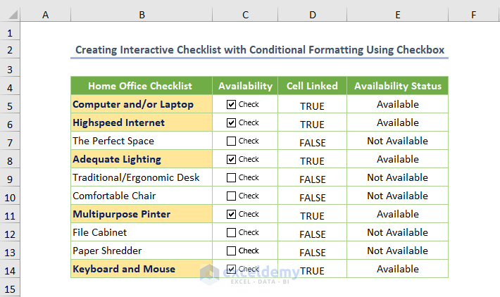
Now, check the interactive checklist by clicking over the box C5 cell, you’ll get the highlighted B5 cell and the status as Available within seconds.
Read More: How to Apply Conditional Formatting Using Checkbox in Excel
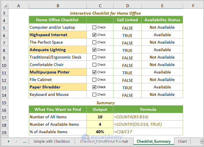
3. Add Checkbox to Create an Interactive Checklist with Summary
Besides, if you want to find an overall summary of the checklist, you may also execute that easily.
For example, you may need to find the number of all items, the number of checked (available) items, and the percentage of the available items.
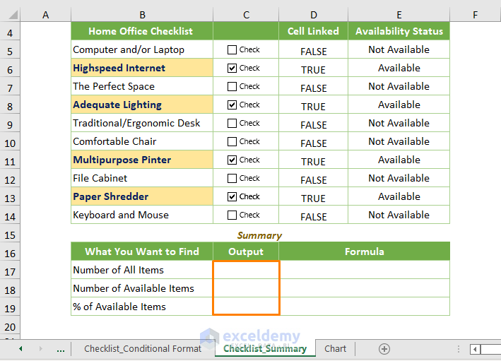
To find the number of all items, the following formula will be in the C17 cell.
=COUNTA(B5:B14)
To find the number of available items using the COUNTIF function, the formula may be used in the C18 cell.
=COUNTIF(D5:D14, TRUE)
Here, D5:D14 is the cell range of the Linked Cell.
Moreover, the formula for getting the percentage will be-
=C18/C17
C18 is the number of available items whereas C17 is the number of total items.
Additionally, you have to turn on the percentage format in the C18 cell from the Format Cells (just press CTRL + 1).
So the summary of the checklist will be like the following.
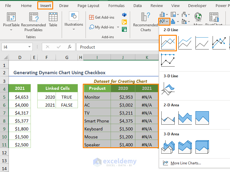
4. Add Checkbox to Generate Dynamic Chart
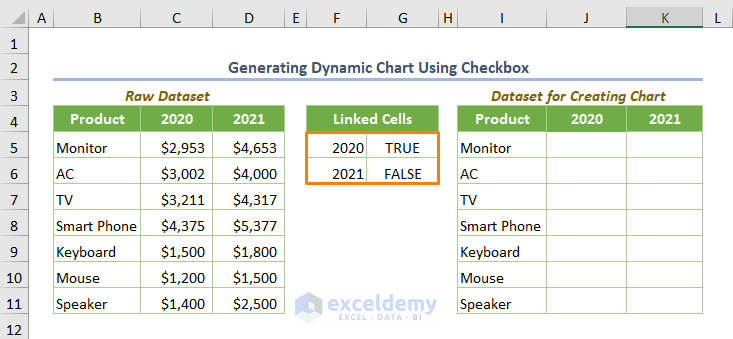
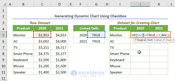
Last but not least, you might produce a dynamic chart using the checkbox in Excel. Let’s see the following dataset where yearly (2020 and 2021) product sales are provided with the product name. First, create the linked cells for two years. For example, G5 is for 2020 and G6 is for 2021.
Then insert the following formula in the J5 cell for I5:I11 cells and use the Fill Handle Tool.
=IF($G$5=TRUE,C5,NA())
Similarly, the formula for 2021 year will be-
=IF($G$6=TRUE,C5,NA())
At this stage, add two checkboxes namely 2020 and 2021. And link the checkbox with the $G$5 cell for 2020 and $G$6 cell with the 2021 checkbox.
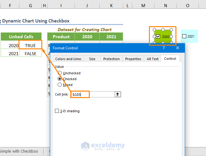
Therefore, generate a 2-D Line chart from the Charts ribbon in the Insert tab. Prior to doing that, select the I4:K11 cell range.
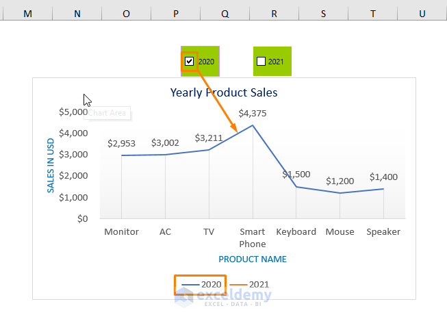
Right now, look closely at the following chart where the data will be automatically updated and the chart shows the data only for 2020 as the box of the year is checked.
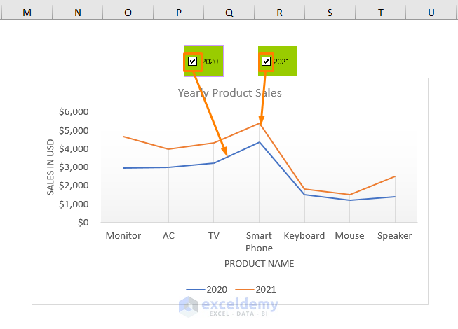
But if you want to check the two boxes simultaneously, you’ll get two line charts for two different years.
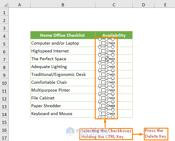
How to Delete a Checkbox in Excel
Though it’s not the focus of the article, still I’m showing it to ease your task. To delete a single checkbox, only select the box and press the DELETE key. Contrarily, you have to select the checkboxes and keep holding the CTRL key if you want to delete the multiple checkboxes. Finally, press the DELETE key.
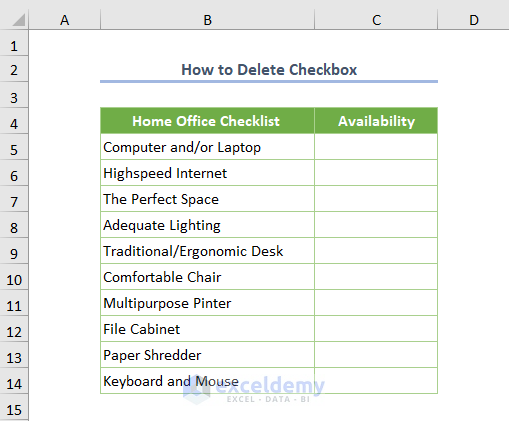
Now, the checkboxes are deleted as shown in the below image.
Read More: How to Remove Checkboxes from Excel
Download Practice Workbook
Conclusion
That’s the end of today’s session. And this is all about the basics, examples of the checkbox including the methods on how to add it in Excel. I strongly believe this article will enrich your Excel learning. Anyway, if you have any queries or recommendations, don’t forget to share them in the comments section below.
Related Articles
- How to Align Checkboxes in Excel
- How to Resize Checkbox in Excel
- How to Count Checkboxes in Excel
- How to Group Checkboxes in Excel
- How to Filter Checkboxes in Excel
<< Go Back to Excel CheckBox | Form Control in Excel | Learn Excel

