In this tutorial, I am going to share with you 3 practical examples of how to apply conditional formatting using a checkbox in Excel. You can easily apply these examples in any set of data to perform various task-checking operations. To achieve this task, we will also see some useful features that might come in handy in many other Excel-related tasks.
How to Apply Conditional Formatting Using Checkbox in Excel: 3 Practical Examples
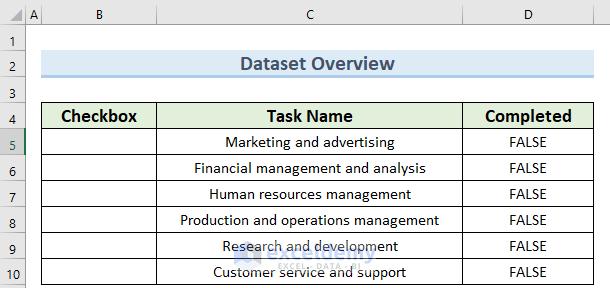
We have taken a concise initial dataset to explain the steps clearly. The dataset has approximately 7 rows and 3 columns. Initially, we are keeping all the cells in General format. For all the datasets, we have 3 unique columns which are Checkbox, Task Name, and Completed. However, we may vary the number of columns later if that is needed. Also, initially, we have inserted the value as FALSE for all the tasks.
1. Adding Strikethrough Formatting
You may format cells in Excel based on certain conditions using Conditional Formatting. Strikethrough formatting, which is a line through the text in a cell, is one style of formatting that might be helpful. This tutorial will teach you how to format Excel cells with strikethrough using checkboxes. You may quickly and simply strike through text in a cell with a single click by adding a checkbox in your Excel worksheet and setting up a conditional formatting rule. This is a practical technique to keep track of work or designate it as finished.
Steps:
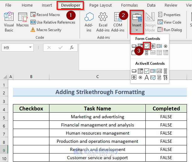
- First, go to the Developer tab and click on the Insert drop-down as in the image below.
- Now, under Form Controls, click on Check Box.
- Consequently, you should see a + symbol on your worksheet.
- Now, click and drag this + symbol on the cell where you want to insert the checkbox.

- As a result, you should get a checkbox with some default text inside.

- Next, delete the default text and copy the checkbox to the other cells below.

- After that, right-click on any of the checkboxes and select Format Control.
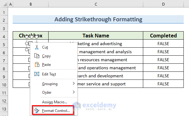
- Here, enter the cell reference that you want to link to the checkbox and click OK.

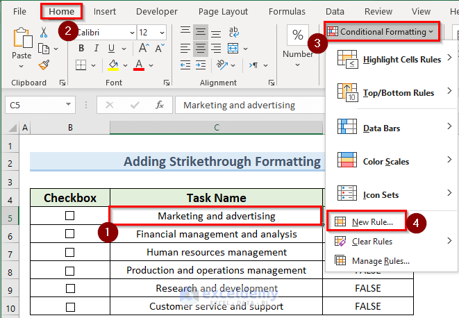
- Now, select the cell that has the name of the task and navigate to the Home tab as in the image below.
- Next, under Conditional Formatting, click on New Rule.
- Then, in the new window, select Use a formula to determine which cells to format and enter the cell reference that you inserted a few steps ago.
- Now, click on Format.

- Here, under the Font tab, check Strikethrough.
- Now, see the preview and click OK.

- Again, confirm the preview and click OK.

- Finally, when you check the checkbox in cell B5, it should strike the value in cell C5.
- Similarly, you can follow the above steps for the other checkboxes.

2. Applying Fill Color Formatting
Excel’s Conditional Formatting feature enables you to format cells based on specific conditions. Fill color, which is a solid color applied to the background of a cell, is one type of formatting that can be employed. In this article, we’ll change cell color if the Checkbox is checked with Conditional Formatting. You may swiftly and easily change the fill color of a cell with a single click by including checkboxes in your worksheet and setting up a conditional formatting rule. This might be a useful technique for emphasizing key information or graphically organizing your data.
Steps:
- To begin with, complete the initial steps of method 1.
- Then, in the Format Cells window, go to the Fill tab and select any fill color.
- Here, see the preview color and click OK.

- Finally, click on any of the checkboxes for which you completed a task and it should have a fill color as you selected just above.

3. Implementing Text Greying Formatting
With Excel’s Conditional Formatting, you may format cells in accordance with specific conditions. Making the text in a cell appear lighter or greyed out is one style of formatting that can be useful. We will learn how to use a checkbox in this article to apply text-graying conditional formatting to Excel cells. You may quickly and simply gray out the text in a cell with just the press of a button by including checkboxes in your worksheet and creating a conditional formatting rule. This might help you visually distinguish between activities that have been accomplished and those that have not, or it can help you emphasize or underline key details.
Steps:
- Firstly, complete the beginning steps of method 1.
- Next, in the Format Cells window, go to the Font tab and select a font color under the Color drop-down as in the image below.
- Then, click OK.

- As a result, if you now click on the checkbox you just formatted, it should grey out the specific task.

Download Practice Workbook
You can download the practice workbook from here.
Conclusion
I hope that you were able to apply the methods that I showed in this tutorial on how to apply Conditional Formatting using a Checkbox in Excel. As you can see, there are quite a few ways to achieve this task. So wisely choose the method that suits your situation best. If you get stuck in any of the steps, I recommend going through them a few times to clear up any confusion. If you have any queries, please let me know in the comments.
Related Articles
- How to Align Checkboxes in Excel
- How to Link Multiple Checkboxes in Excel
- How to Resize Checkbox in Excel
- How to Count Checkboxes in Excel
- How to Group Checkboxes in Excel
- How to Filter Checkboxes in Excel
- How to Remove Checkboxes from Excel
- How to Add Checkbox in Excel without Using Developer Tab
<< Go Back to Excel CheckBox | Form Control in Excel | Learn Excel
Get FREE Advanced Excel Exercises with Solutions!
