How to Filter Checkboxes in Excel (with Easy Steps)

In this article, we will demonstrate how to add checkboxes in Excel and then Filter them.

Step 1 – Enable Developer Tab

Before we delve into Filtering the Checkboxes, we’ll add them to the sheet first.

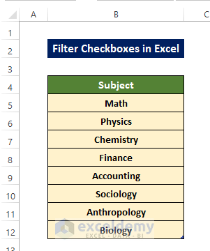
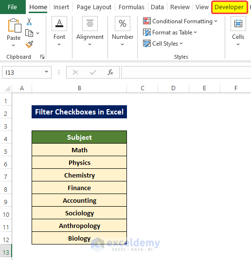
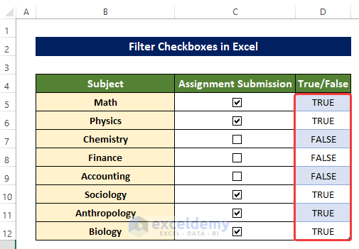
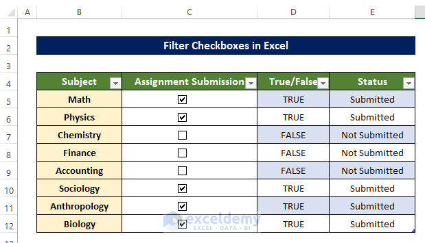
Suppose we have the below subjects in a dataset. We will add checkboxes so that we can monitor the submissions.

Add Developer Tab to Filter Checkboxes in Excel

We add checkboxes to a worksheet in Excel from the Developer tab on the ribbon, which by default is disabled. If you see the Developer tab on your ribbon, you can skip this step, otherwise you’ll need to enable it.

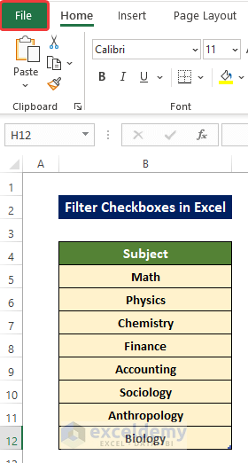
Click on the File command in the top left corner of the sheet.

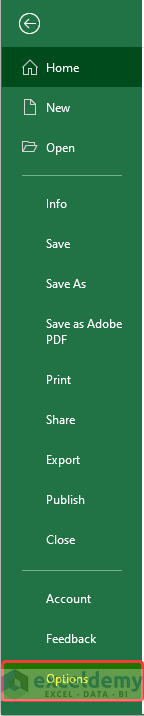
In the menu that opens, click on Options.

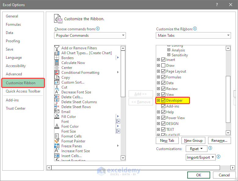
In the Excel Options dialog box that opens, click on Customize Ribbon.
On the right side of the menu list, check if the Developer checkbox appears.
If it is not there, add the Developer option from the left menu list.

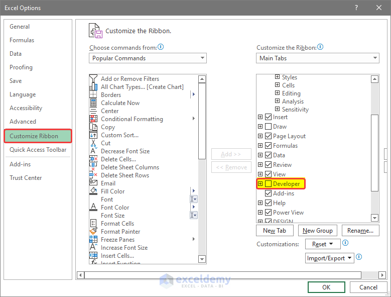
Check the Developer option and click OK.

Now the Developer tab appears on the ribbon.

Step 2 – Add Checkboxes from the Developer Tab

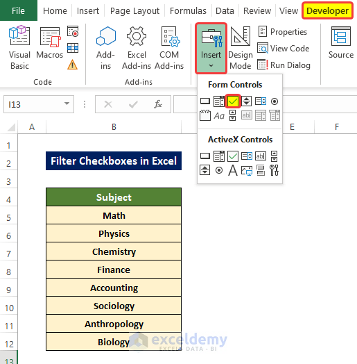
Click on the Developer tab then on Insert.
From the dropdown menu, click on the checkbox icon.

A drawing icon will appear on the sheet.

Carefully draw the Checkbox boundaries. Try to match the edge of the cell with the draw icon.

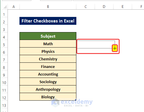
After carefully drawing out the Checkbox, click anywhere on the sheet.

Your checkbox is present.

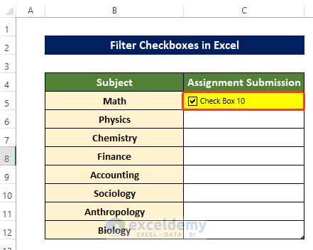
Right-click on the box and from the context menu, click on Edit Text.

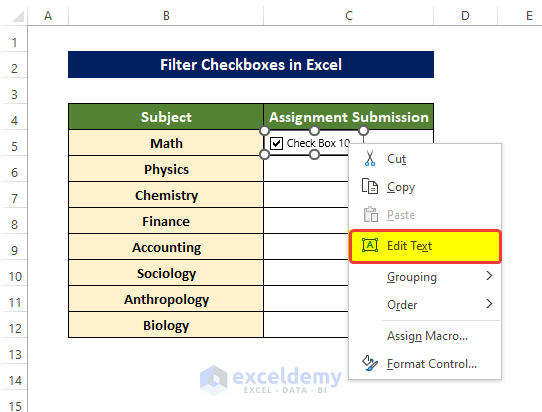
Remove all the text.

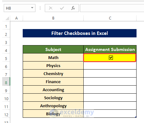
The Checkbox will look something like the one below.

Right-click on the Checkbox and from the context menu, click on Copy.

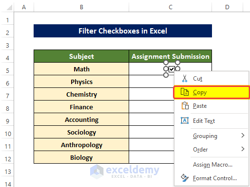
Select cell C5, and right-click again.
From the context menu, click on the Paste icon.

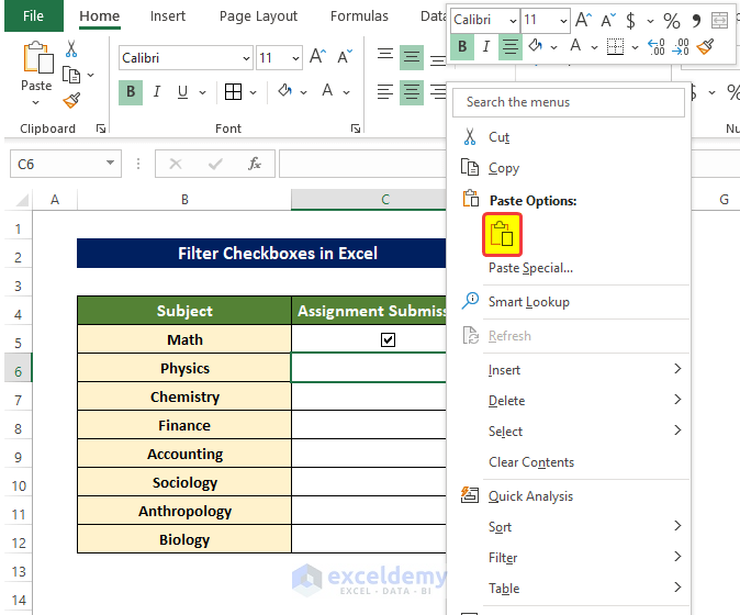
The Checkbox is pasted in cell C5.

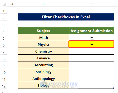
Repeat the same process for the rest of the cells.

After copying the Checkboxes, the table will look somewhat like the one below.

Note

The drawing of the Checkbox areas needs to be precise, matching the cell boundaries. Otherwise, when copied down to the cells below, they could overlap and create visual irritation.

Step 3 – Link Checkboxes with Adjacent Cells

We can add a column stating whether the submission of the assignments is done or not using the IF function.

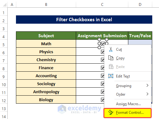
Select the topmost Checkbox and right-click on it.
From the context menu, click on Format Control.

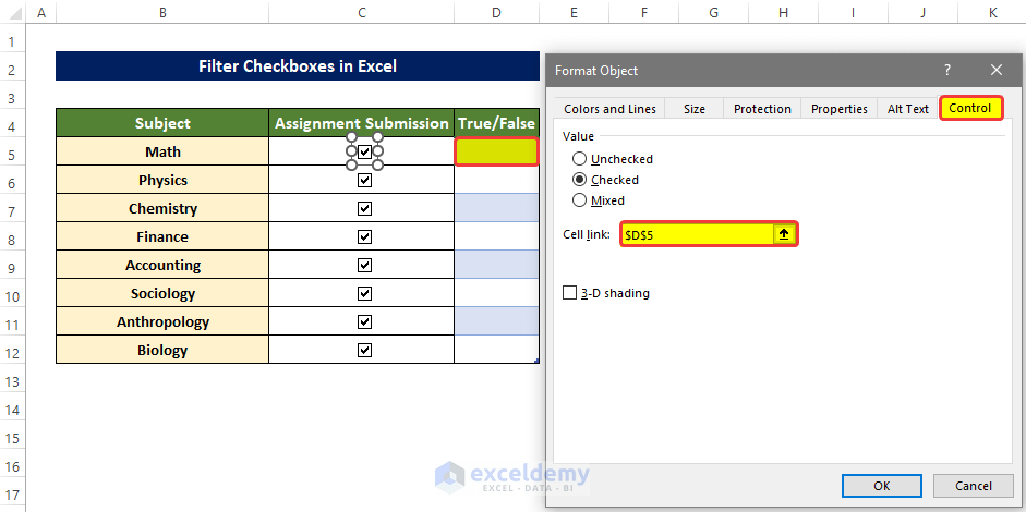
In the Format Object window, click on Cell Link from the Control group.
Click OK.

The cell is now linked with the check box.

Repeat the same process for the rest of the cells.

In cell E5, enter the following formula:

=IF(D5=TRUE,"Submitted","Not Submitted")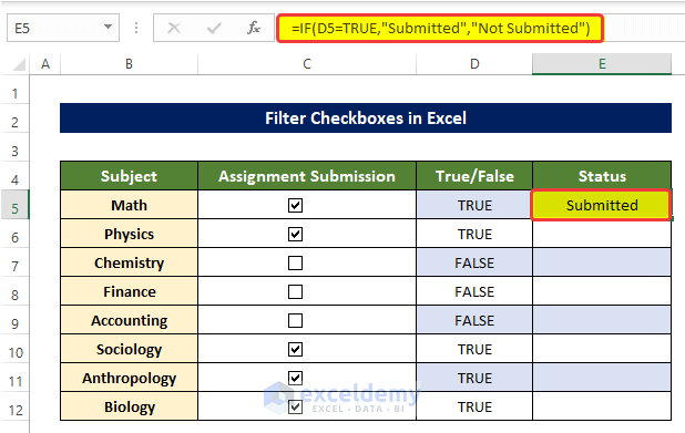

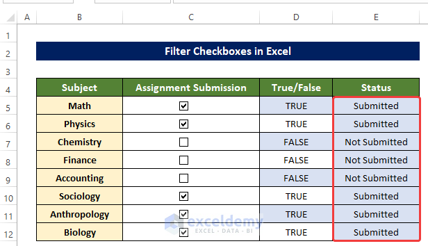
Drag the Fill Handle down to cell E12.

This will fill the range of cells E5:E12 with the submission status of each student.

Step 4 – Create Table

Now we will turn the data range into a table, where a Filter will be applied by default.

Select the range of cells B5:E12.
From the Insert tab, click on the Table in the Tables group.

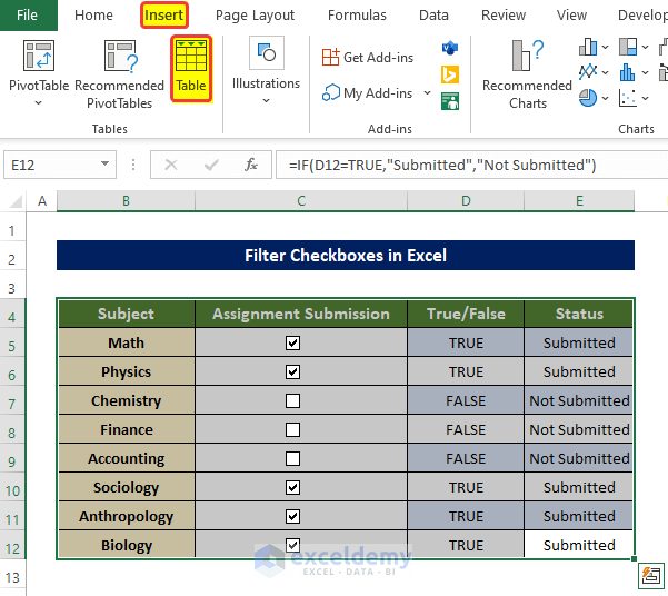
The whole range of cells will be converted to a table with a Filter icon on each table header.

Step 5 – Filter Checkboxes

Now we can Filter the Checkboxes based on their status.

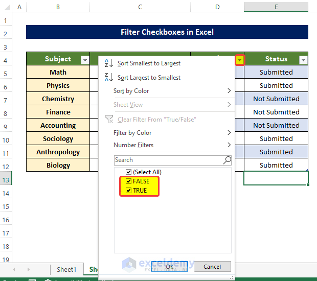
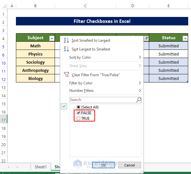
Click on the Filter drop-down icon on the True/ False table header.

True and False selected.

Uncheck the False box and click OK.

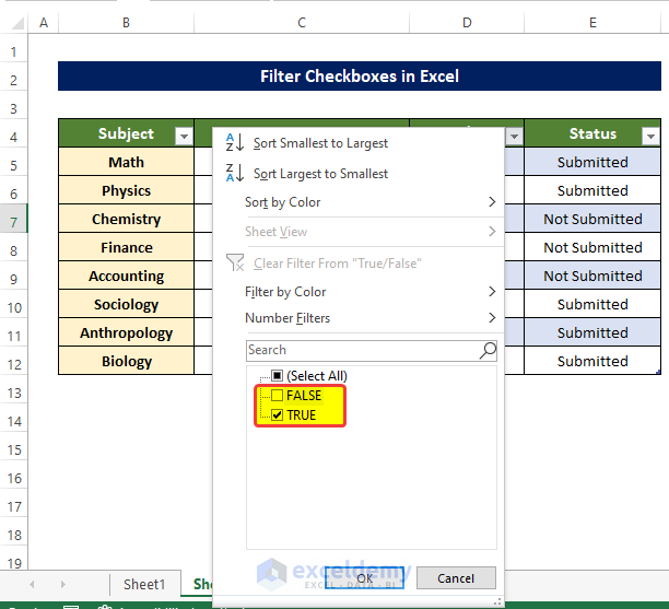
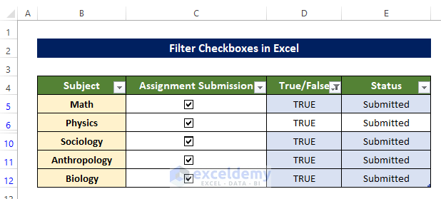
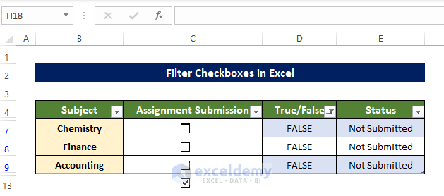
Only entries with True are showing. We effectively Filtered out the entries with False.

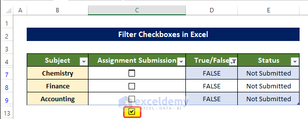
Now check only the False box and click OK.

Only entries with False showing.

Note

Notice that there is an extra checkbox in the cell just below the table. The reason this cell has an extra Checkbox is that Checkboxes are an object. As this Checkbox does not interfere with our ask of Filtering the Checkboxes, it can be ignored.