How to Insert Checkboxes in Excel
Method 1 – Insert a Single Checkbox
Steps
- Go to the Developer tab in the ribbon. If you don’t see the tab, you have to enable the Developer tab.
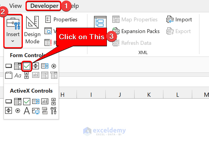
- Click the Insert option. From Form Controls, click on the Checkbox.
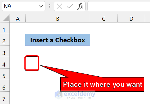
- You will find a plus sign(+) that indicates the checkbox. Place it in any cell.
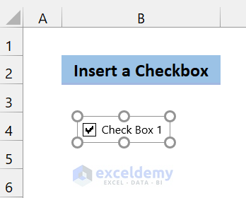
- You will get the following checkbox.
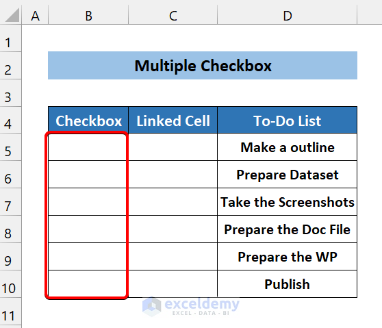
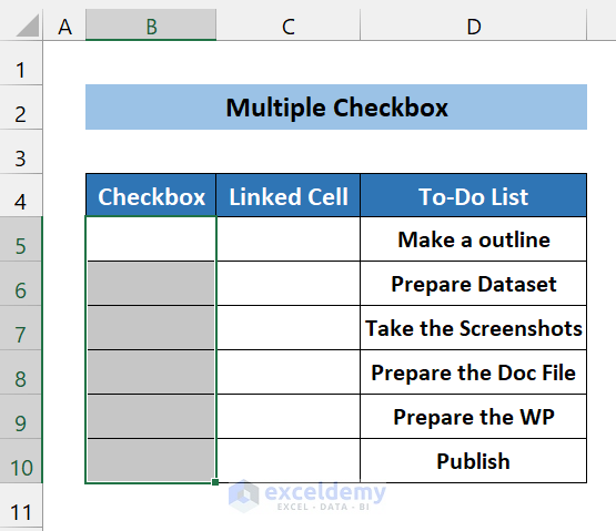
Method 2 – Insert Multiple Checkboxes and Link Them
We’ll fill column B with six checkboxes and link them to the respective cells in column C.
Steps
- Press Alt + F11 on your keyboard to open the VBA editor.
- Select Insert and choose Module.

- Insert the following code:
Sub add_multiple_checkbox()

Dim cell As Range

Dim shape_of_box As CheckBox

  For Each cell In Selection.Cells

    Set shape_of_box = ActiveSheet.CheckBoxes.Add(cell.Left, cell.Top, cell.Width, cell.Height)

    With shape_of_box

      .Text = ""

      .Width = cell.Width

      .LinkedCell = cell.Offset(0, 1).Address

    End With

  Next cell

End

End Sub- Save the file.
- Select the range of cells B5:B10.
- Press Alt + F8 to open the Macro dialog box.
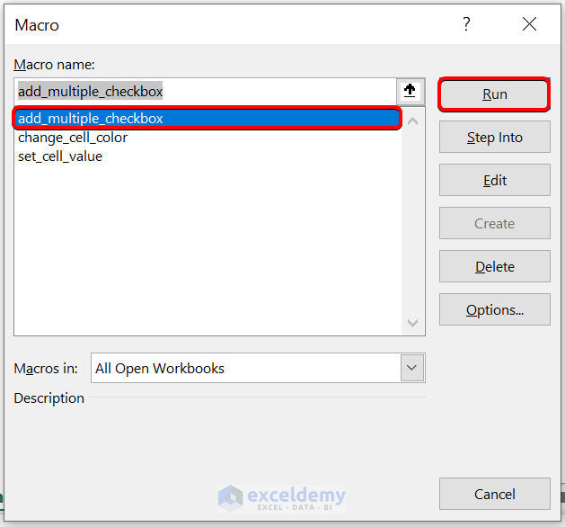
- Select add_multiple_checkbox.
- Click on Run.
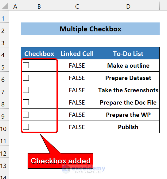
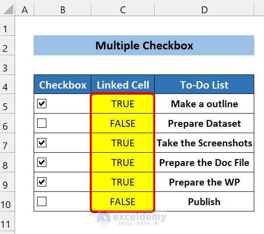
- You’ll get multiple checkboxes in the Checkbox column. You can tick a box and set the adjacent value to TRUE.
Customize the Checkbox in Excel
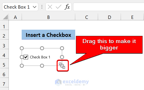
- You can drag the box around the checkbox to make it bigger or smaller:
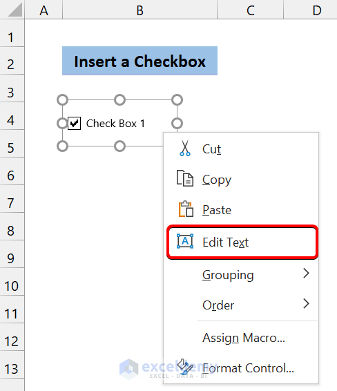
- You can change the “Check Box 1” name to another name. Right-click on the checkbox and choose Edit Text.
Link the Checkbox with a Cell
Steps
- Right-click on the checkbox.
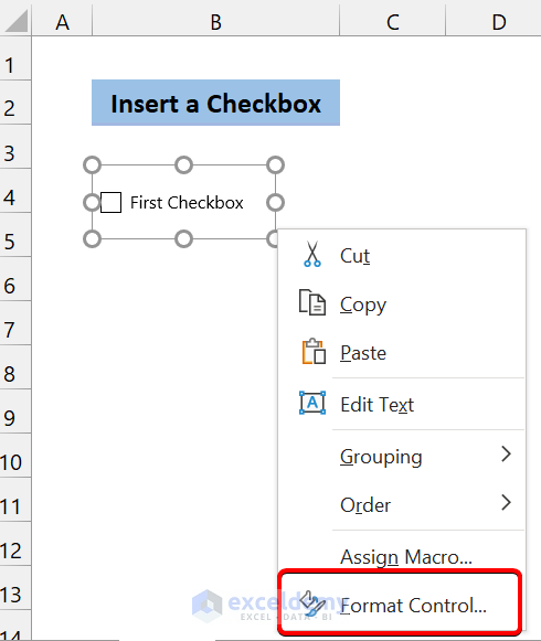
- Click on the Format Control option.
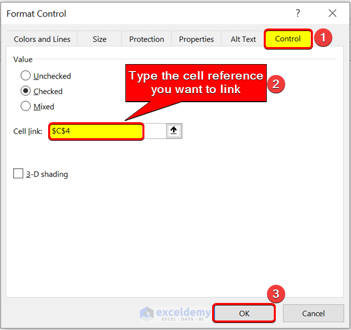
- From the Format Control dialog box, go to the Control tab.
- In the Cell link box, insert or select the cell you want to link with the checkbox.
- Click on OK.
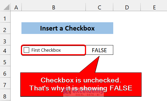
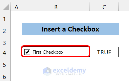
- If you check the box, the value is set to TRUE. Otherwise, it stays FALSE.
How to Change Cell Color in Excel If Checkbox is Checked: 2 Methods
Method 1 – Use Excel Conditional Formatting to Change Color If the Checkbox Is Checked
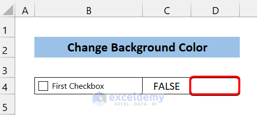
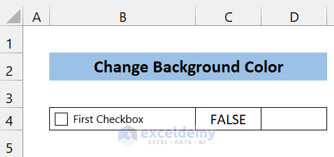
We’ll use a simple dataset with a single checkbox linked to an adjacent cell.
Steps
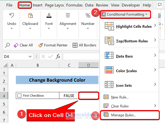
- Click on Cell D4.
- From the Home tab, click on Conditional Formatting.
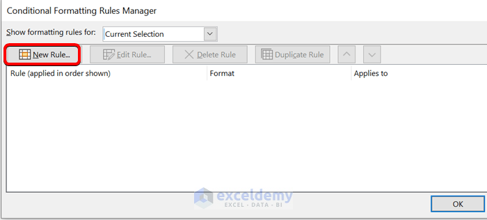
- Click on New Rule, or click on Manage Rules and select New Rule.
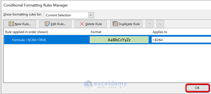
- Select the option Use a formula to determine which cells to format.
- Insert the following formula in the box:
=$C$4=TRUE
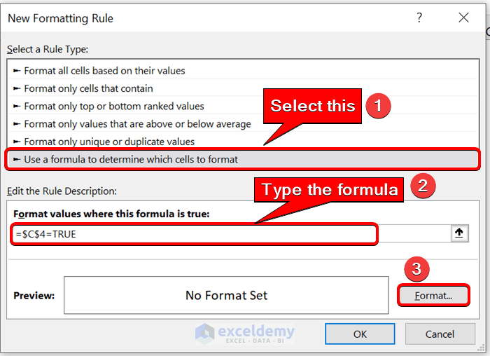
- Click on Format.
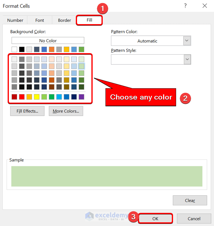
- Click on Fill.
- Choose any color that’s not white and click on OK.
- Your formula and the background color are set. Click on OK again.
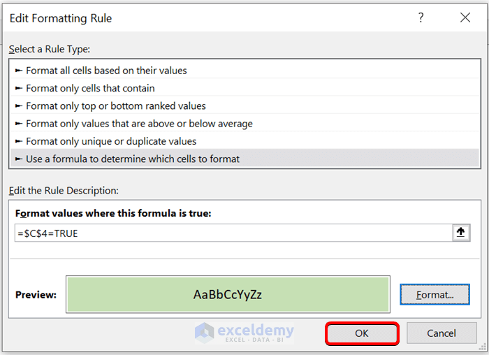
- If you’ve used Manage Rules, you’ll need to click OK again.
- Here’s the result.
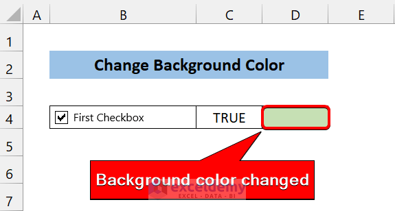
- Tick the checkbox and the color changes.
Method 2 – Use Excel VBA to Change Cell Color If the Checkbox Is Checked+
Steps
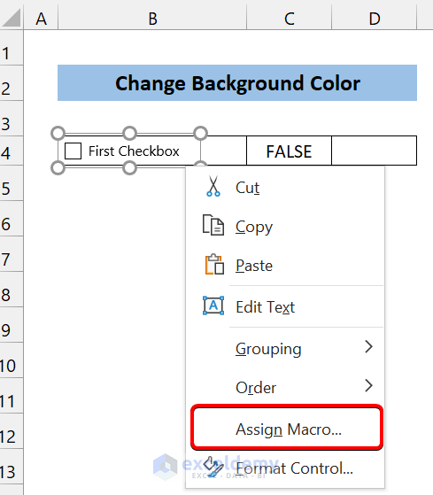
- Right-click on the checkbox.
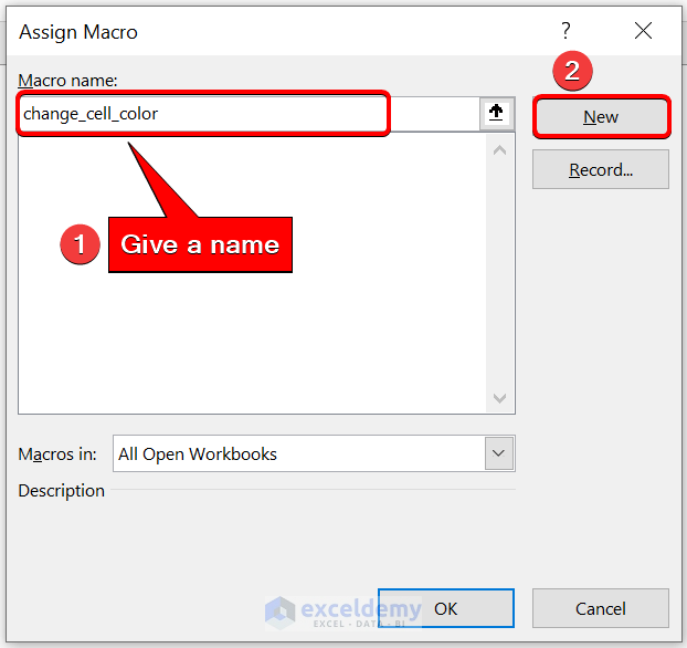
- Click on Assign Macro.
- Give the Macro a name.
- Click on New. It will open the Visual Basic Editor.
- Insert the following code:
Sub change_cell_color()

Dim rng As Range

Set rng = Range("D4")

If Range("C4").Value = True Then

    rng.Interior.Color = vbRed

Else

    rng.Interior.Color = xlNone

End If

End Sub- Save the file.
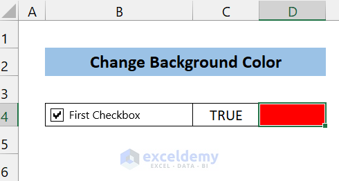
- If you check the box, it will change the cell color to Red.
Set a Cell Value in Excel If the Checkbox Is Checked
We’ll use the same dataset.
- Right-click on the checkbox and click on Assign macro.
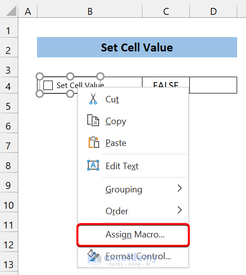
- Name the macro and click on New in the Macro box.
- Insert the following code in the editor.
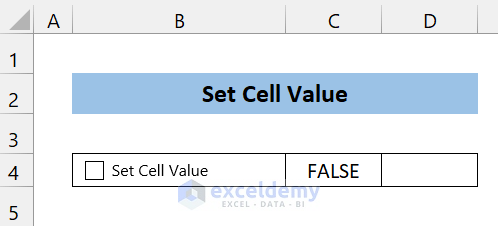
Sub set_cell_value()

Dim rng As Range

Dim c As Range, cell_value As String

Set rng = Range("D4")

If Range("C4").Value = True Then

    rng.Value = "Done!"

Else

    rng.Value = ""

End If
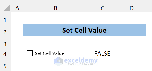
End Sub- Save the file. You can see no value yet.
- Click on the checkbox and you will see a value in Cell D4:
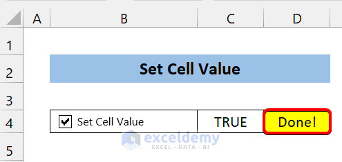
You can modify the value by changing the text in the following code line:
rng.Value = "Done!"
Read More: What Can You Do with Cell Value If Checkbox Is Checked in Excel?
Things to Remember
✎ You can also insert a checkbox from ActiveX controls.
✎ You can also change the color of multiple cells if the checkbox is checked. Select the range of cells you want to color and follow a similar process in Conditional Formatting.
✎ You must save the file in the .xlsm format.
Download the Practice Workbook
Related Articles
- If Checkbox Is Checked Then Apply Formula in Excel
- VBA to Check If CheckBox Is Checked in Excel
- Excel VBA: Form Control Checkbox Value
<< Go Back to Excel CheckBox | Form Control in Excel | Learn Excel
Get FREE Advanced Excel Exercises with Solutions!
