How to Insert and Use Excel Form Control

Written by Mehedi Hassan

Last updated: May 6, 2024

Turning On the Developer Tab

Go to the File tab in the ribbon. Click on it, and Excel will show you the Backstage view.

Click on Options in the left-down corner.

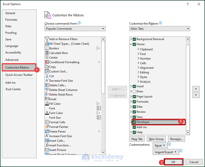
A box will appear.
Select Customize Ribbon.
At Main Tabs, check the Developer box.
Press OK.

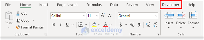
You will now see the Developer tab.

Choosing the Desired Form Control

Go to the Developer tab.
Select the Enter option from the Controls group.

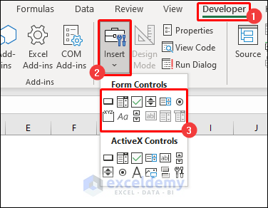
From the drop-down list, you can select any control button from the Form Controls section.

How to Use Form Controls in Excel

1. Form Control: Button

Steps:

Go to the Developer tab.
Select the Insert option from Controls.
From the drop-down, select the Button command from Form Controls.

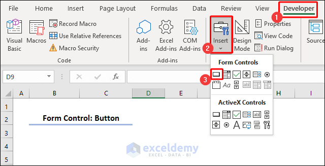
The cursor will now look like a plus (+) sign.

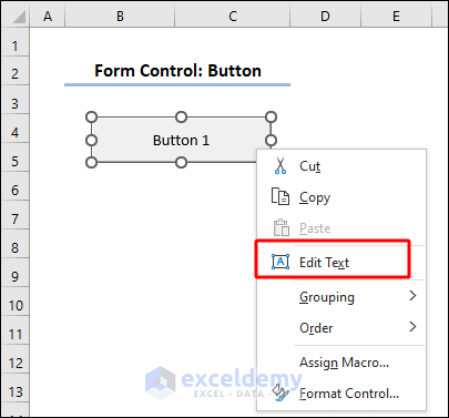
Drag the plus (+) sign and create a button.
Set a name for the button.
Right-click on the button and select Edit Text from the Context Menu.

Right-click on the button and select Assign Micro.

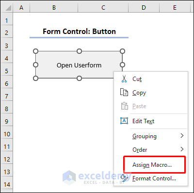
Select New in the Assign Macro dialogue box.

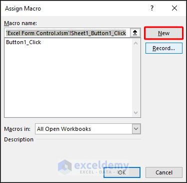
A VBA module window will appear.
Enter the following code into the module and close it.

Sub Button1_Click()
UserForm1.Show
End Sub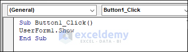

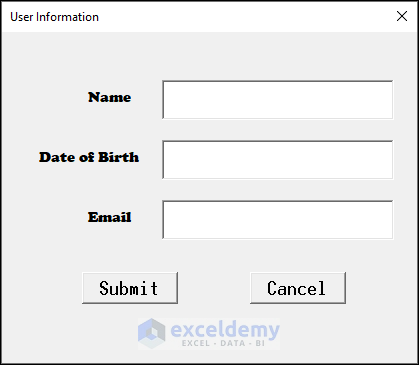
Note: We’ve already created a Userform, and the code will activate when the button is clicked.

Click the button, and you will see the UserForm.

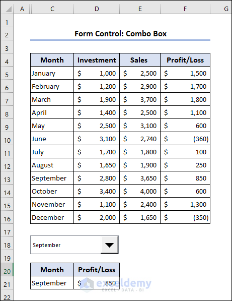
2. Form Control: Combo Box

Steps:

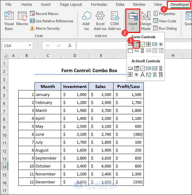
Go to the Developer tab.
Select the Insert option from Controls.
From the drop-down, select the Combo Box from Form Controls.

The cursor will now look like a plus (+) sign.

Drag the plus (+) sign and create a box.
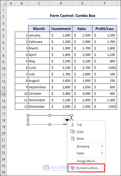
To enlist the months, right-click on the box and select Format Control.

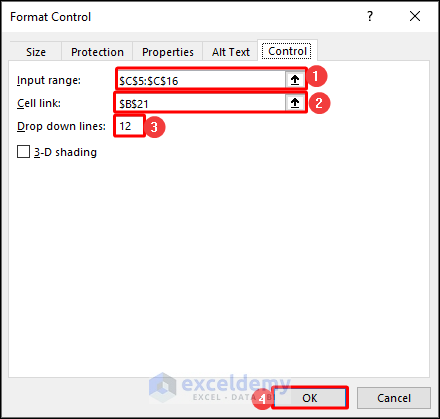
In the Control tab of the Format Control dialogue box, put $C$5:$C$16 in the Input range.
When you select a month, the serial number of that month will be displayed in a cell. Insert $B$21 on the Cell link box.
Enter 12 to the Drop down lines box and press OK.

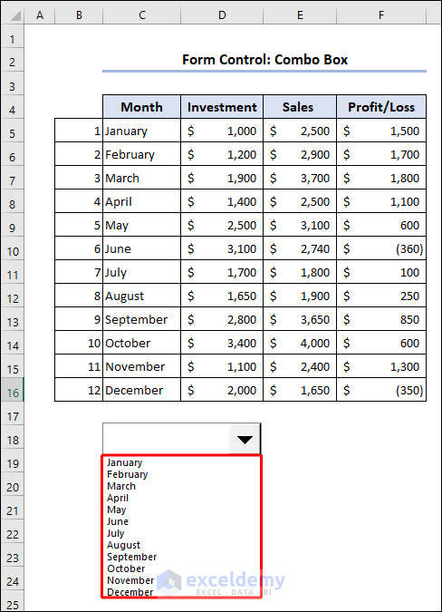
The months are now displayed in the combo box.

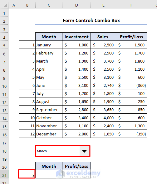
Select March, and the serial number will be displayed in cell B21.

To get the month you selected in the combo box in cell C21, use this formula based on the VLOOKUP function and press Enter.

=VLOOKUP($B$21,$B$5:$F$16,2,TRUE)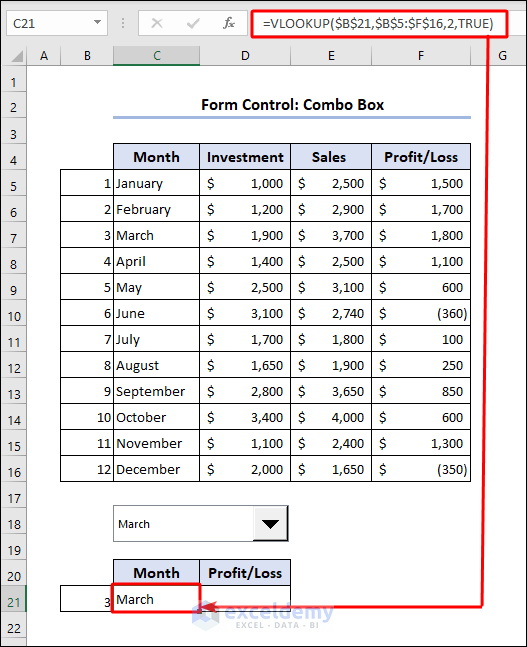

To get the Profit/Loss for the respective month you selected in the combo box in cell D21, use this formula based on the VLOOKUP function and press Enter.

=VLOOKUP($B$21,$B$5:$F$16,5,TRUE)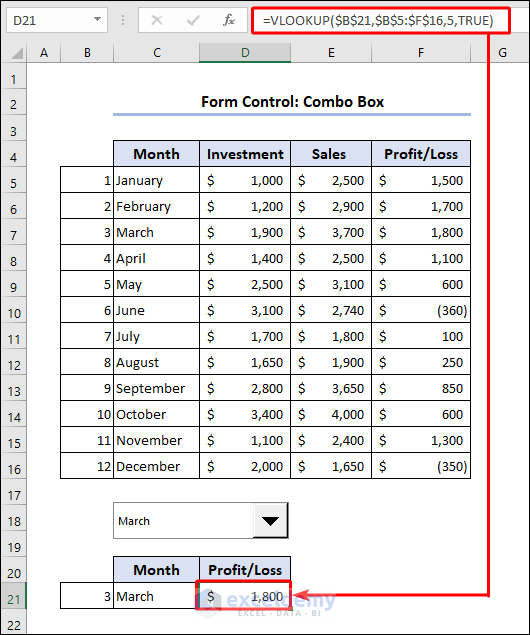

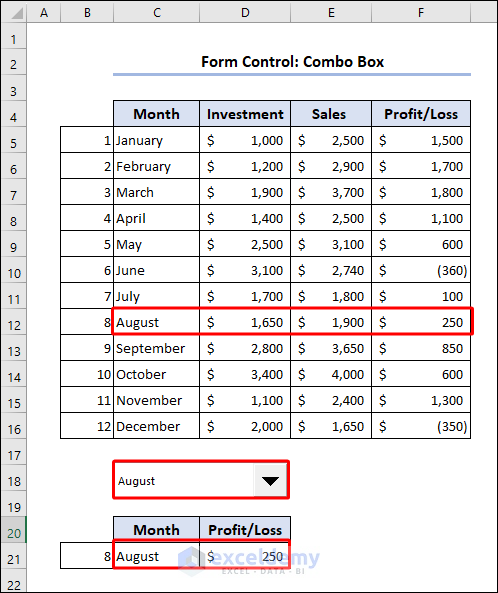
Select August from the combo box. The related data will be displayed in the second table.

To hide column B for better presentation, right-click on the column header.
From the Context Menu, select Hide.

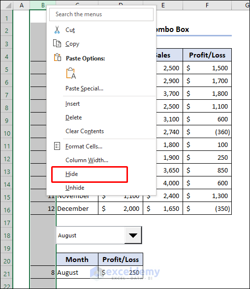
You now have a dynamic dataset with a functioning combo box.

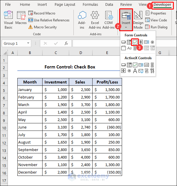
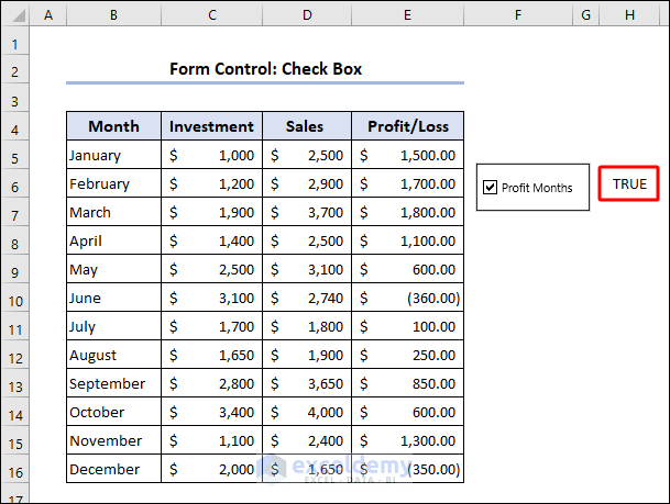
3. Form Control: Check Box

Steps:

Select the Check Box from Form Controls.

The cursor will look like a plus (+) sign.

Drag the plus (+) sign and create a box.
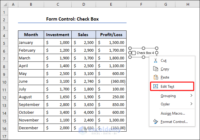
Name the box.
Right-click on the box and select Edit Text from the Context Menu.

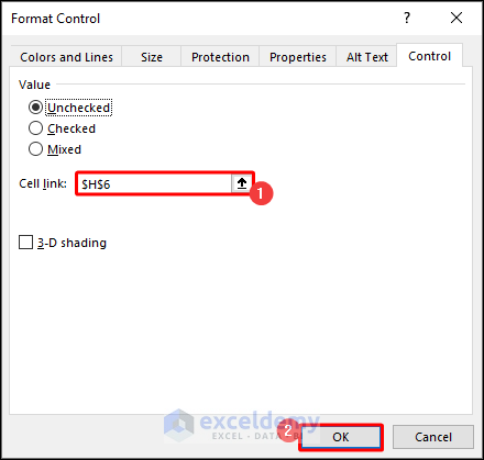
To link a cell for the check box, right-click on the box and select Format Control.

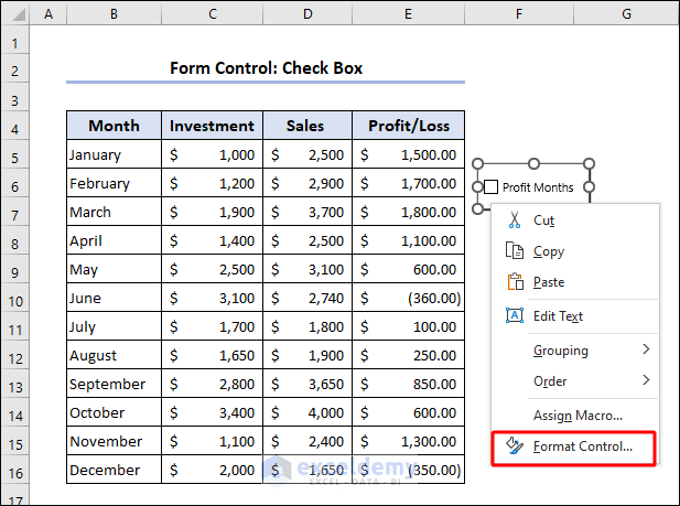
When you check/uncheck the Check Box, a cell will show TRUE/FALSE. To link that cell, enter $H$6 in the Cell link box in the Control tab of the Format Control dialogue box.
Press OK to close the window.

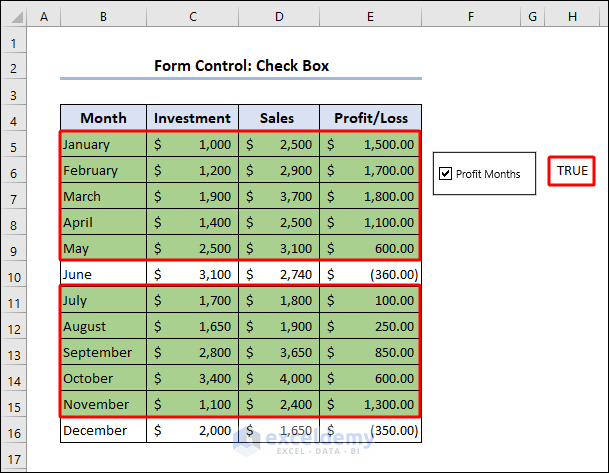
If you check the box, you will notice cell H6 will show as TRUE.

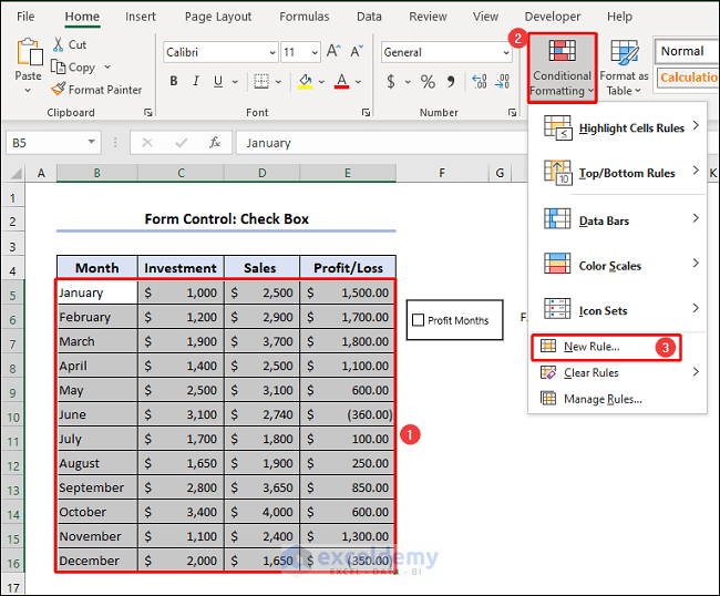
To link this Check Box with our table, go to the Home tab.
From Styles, choose the Conditional Formatting drop-down menu.
Select New Rule.

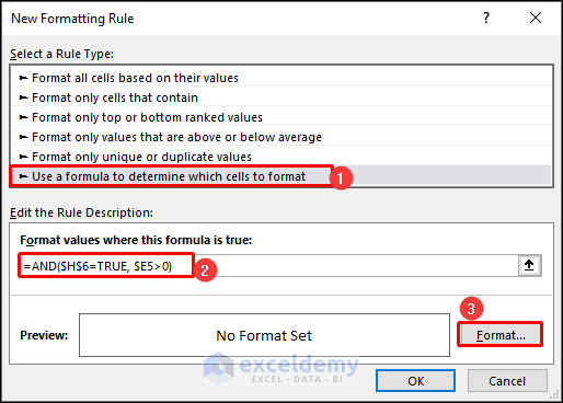
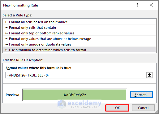
In the New Formatting Rule window, choose Use a formula to determine which cells to format from the Select a Rule Type bar.
Enter the following formula in the Edit the Rule Description box:

=AND($H$6=TRUE, $E5>0)

To choose a Fill color, click Format.

Select the Fill tab and the color you want.

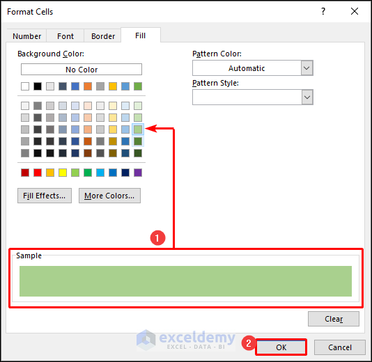
Press OK to take you back to the New Formatting Rule.
Press OK to apply the change.

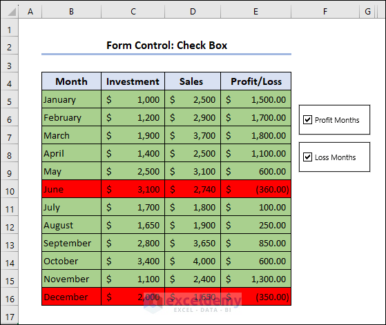
If you check the box, you will see the months that have generated profit have been highlighted.

Create another Check Box following the previous steps and link a cell.
Click Conditional Formatting and enter the following formula:

=AND($H$8=TRUE, $E5<0)

Select a formatting color.

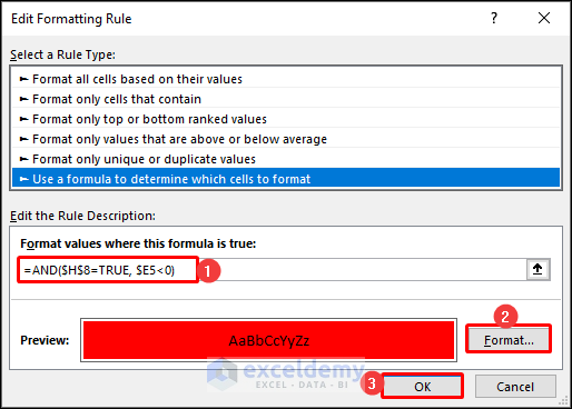
You should have 2 functioning checkboxes.

To hide linked cells for better presentation, right-click on the column header, and from the Context Menu, select Hide.

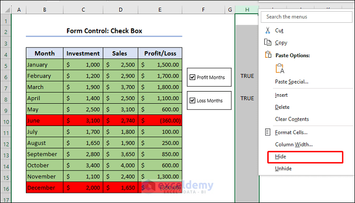
You have a dynamic dataset with 2 functioning checkboxes.

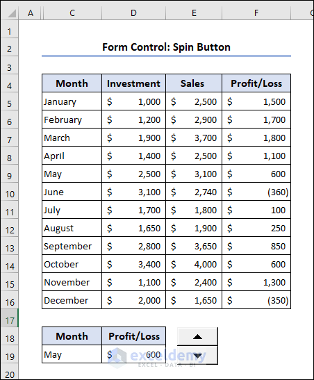
4. Form Control: Spin Button

Steps:

Select the Spin Button from Form Controls.

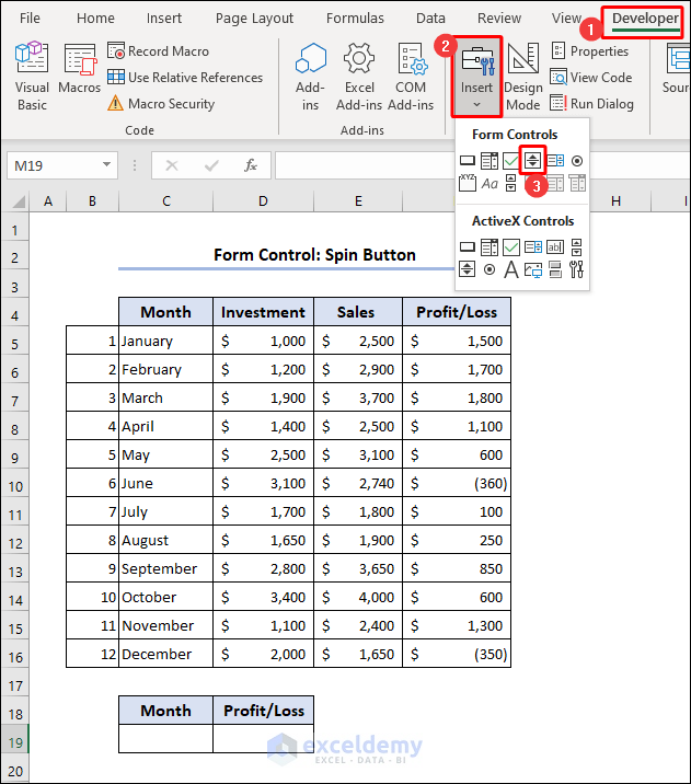
The cursor will look like a plus (+) sign.

Drag the plus (+) sign and create a box.
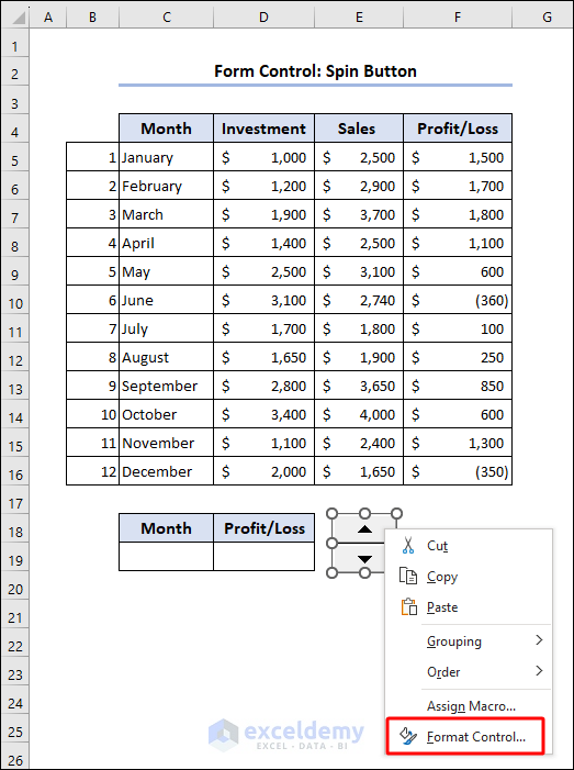
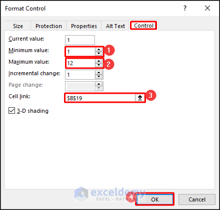
To rotate the months, right-click on the box and select Format Control.

In the Control tab of the Format Control dialogue box, put 1 in the Minimum value box.
Insert 12 as the Maximum value.
When you select a month, the serial number of that month will be displayed in a cell. Enter $B$19 in the Cell link box and press OK.

When you press the up/down button, numbers 1 to 12 will rotate in cell B19.

To get the month rotating as per the button, click on cell C19. Enter the following formula based on the VLOOKUP function, and press Enter.

=VLOOKUP($B$19,$B$5:$F$16,2,TRUE)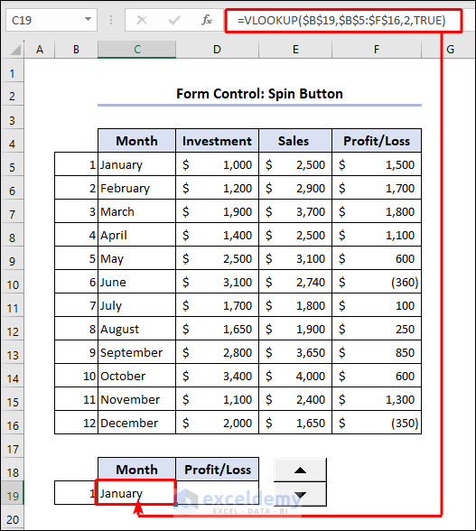

To get the Profit/Loss for the respective month in cell D19, enter the following formula based on the VLOOKUP function and press Enter.

=VLOOKUP($B$19,$B$5:$F$16,5,TRUE)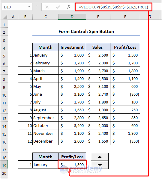

Click the down button, and the Month and respective Profit/Loss will rotate.
To hide column B for better presentation, right-click on the column header, and from the Context Menu, select Hide.

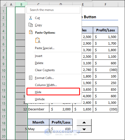
You have a dynamic dataset with a functioning Spin button.

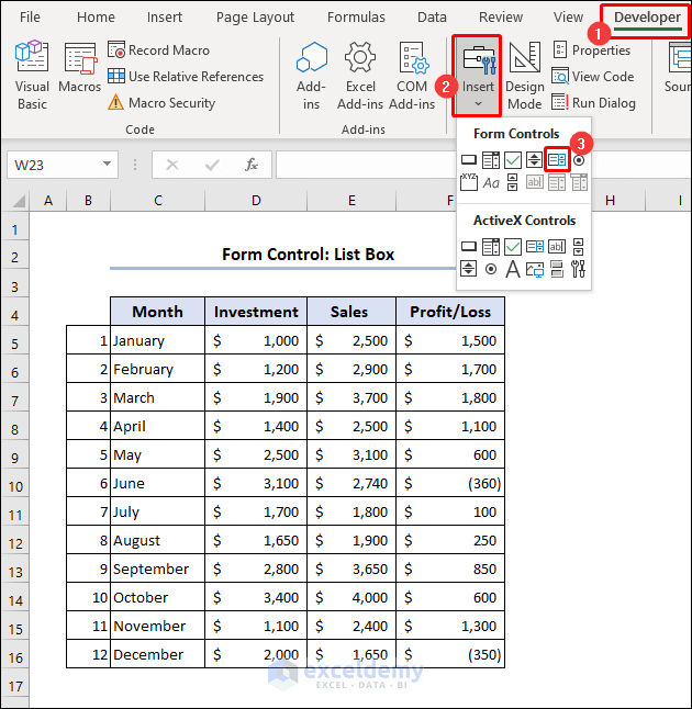
5. Form Control: List Box

Steps:

Select List Box from Form Controls.

The cursor will look like a plus (+) sign.

Drag the plus (+) sign and create a box.
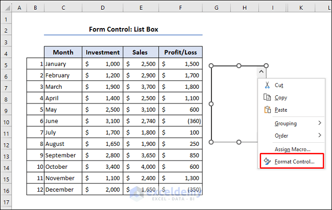
To enlist the months, right-click on the box and select Format Control.

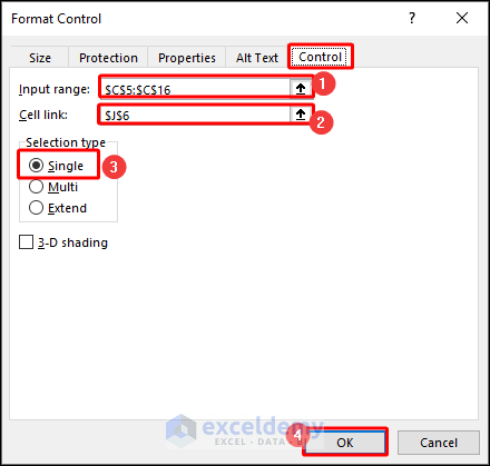
In the Control tab of the Format Control dialogue box, enter $C$5:$C$16 in the Input range.
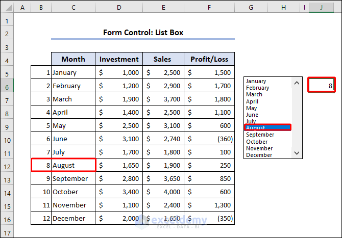
When you select a month, the serial number of that month will be displayed in a cell. Enter $J$6 in the Cell link box.
Select Single in the Selection type and press OK.

The months are enlisted in the combo box.
When you select August, the serial number will displayed in cell J6.

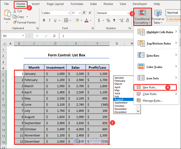
To link this List Box with our table, go to the Home tab.
From Styles, choose the Conditional Formatting drop-down menu.
Select New Rule.

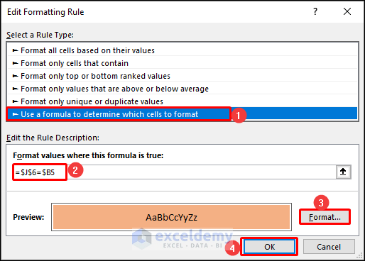
In the New Formatting Rule window, choose Use a formula to determine which cells to format from the Select a Rule Type bar.
Enter the following formula in the Edit the Rule Description box:

=$J$6=$B5

To choose a Fill color, click Format.

Hide the helper columns B and J.

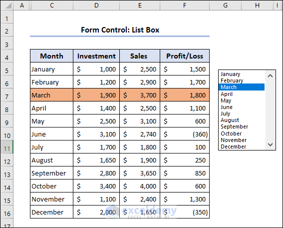
If you select a month from the list box, that month will be highlighted. Here, we selected March, and the corresponding row is highlighted.

6. Form Control: Option Button

Steps:

Select the Option Button from Form Controls.

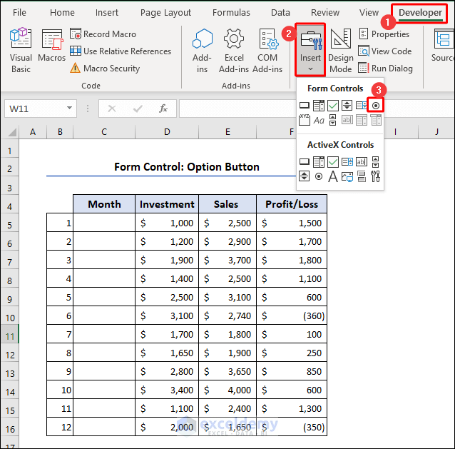
The cursor will look like a plus (+) sign.

Drag the plus (+) sign and create a box.
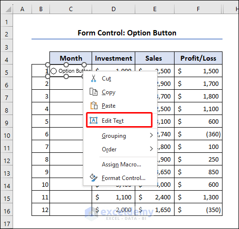
Right-click on the box and select Edit Text from the Context Menu.
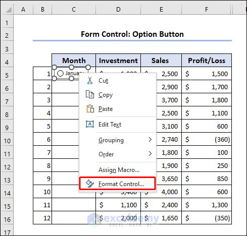
Set a name for the box.

Select the option button, right-click on the button, and select Format Control.

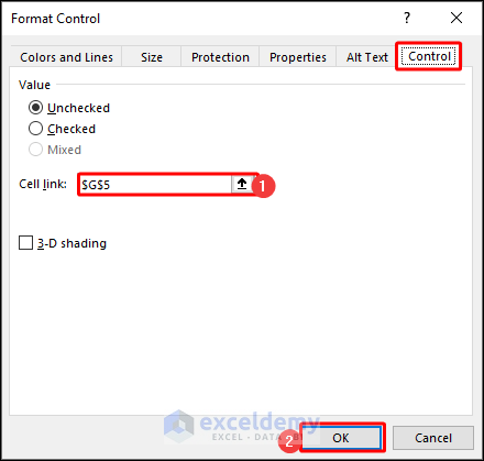
When you check/uncheck the Option Button, a cell will show the Button. To link that cell, enter $G$5 in the Cell link box in the Control tab of the Format Control dialogue box.
Press OK to close the window.

Copy the button and paste it in the next rows.
You will have 12 buttons like this for each month.
When you click a button, cell G5 will show its serial number.

To link these Option Buttons with our table, go to the Home tab.
From Styles, choose the Conditional Formatting drop-down menu.
Select New Rule.

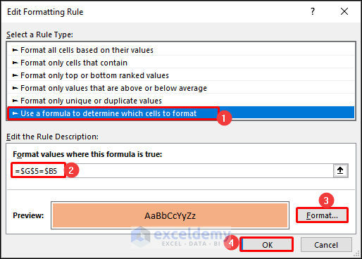
In the New Formatting Rule window, choose Use a formula to determine which cells to format from the Select a Rule Type bar.
Enter the following formula in the Edit the Rule Description box:

=$G$5=$B5

To choose a Fill color, click Format.

Hide the helper columns B and G.

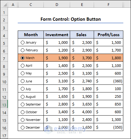
If you select a month, you will see that particular row is highlighted. Here, we selected March, and the corresponding row is highlighted.

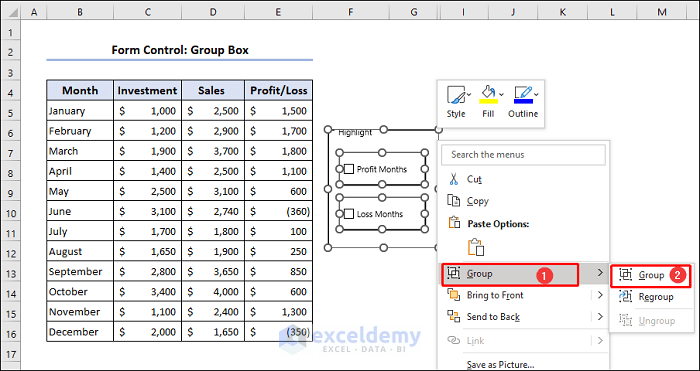
7. Form Control: Group Box

Select Group Box from Form Controls.

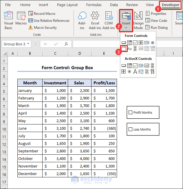
The cursor will look like a plus (+) sign.
Drag the plus (+) sign and create a box over the Check Boxes.
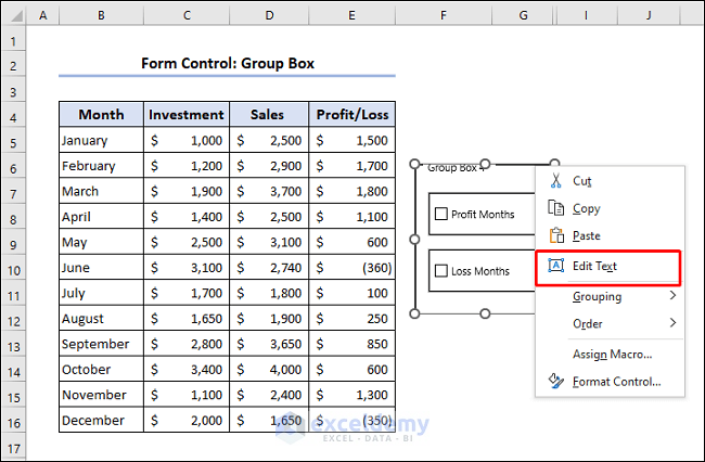
Right-click on the box and select Edit Text from the Context Menu.
Set a name for the box.

To group the controls, select each one by pressing Ctrl and right-click on them.
Select Group from the Context Menu and select Group.

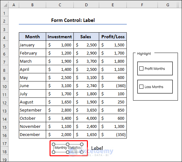
Note: Users can not interact with Group Boxes. They only house other controls.

8. Form Control: Label

Labels don’t interact with users. They only showcase a certain value or text.

9. Form Control: Scroll Bar

Select Scroll Bar from Form Controls.

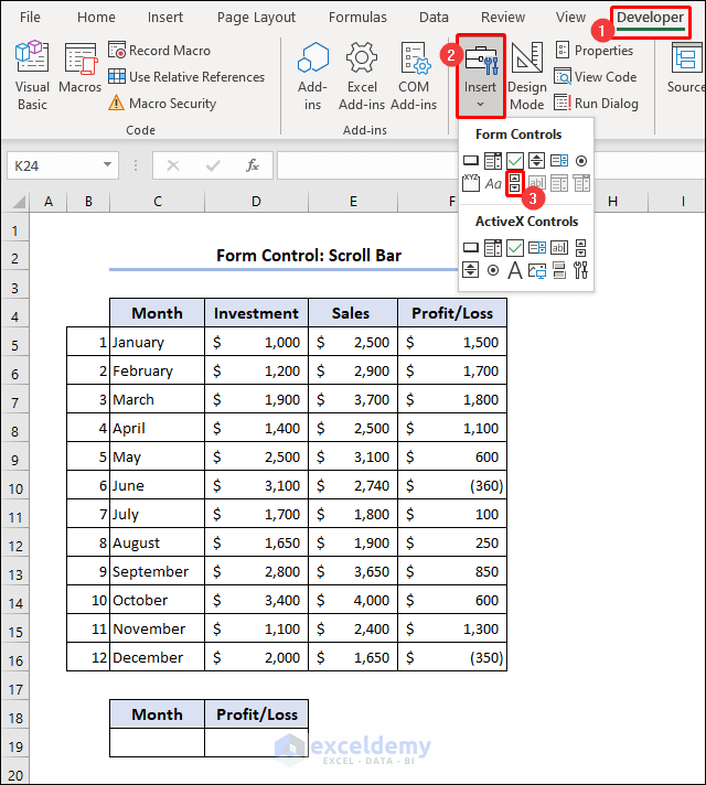
The cursor will look like a plus (+) sign.

Drag the plus (+) sign and create a box.
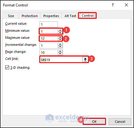
To rotate the months, right-click on the box and select Format Control.

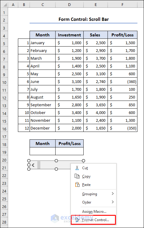
In the Control tab of the Format Control dialogue box, put 1 in the Minimum value box.
Insert 12 as the Maximum value.
When you select a month, the serial number of that month will be printed on a cell. Insert $B$19 in the Cell link box and press OK.

When you press the Scroll Bar, numbers 1 to 12 will rotate in cell B19.

To get the month rotating, as per the button, click on cell C19. Enter the formula based on VLOOKUP function and press Enter.

=VLOOKUP($B$19,$B$5:$F$16,2,TRUE)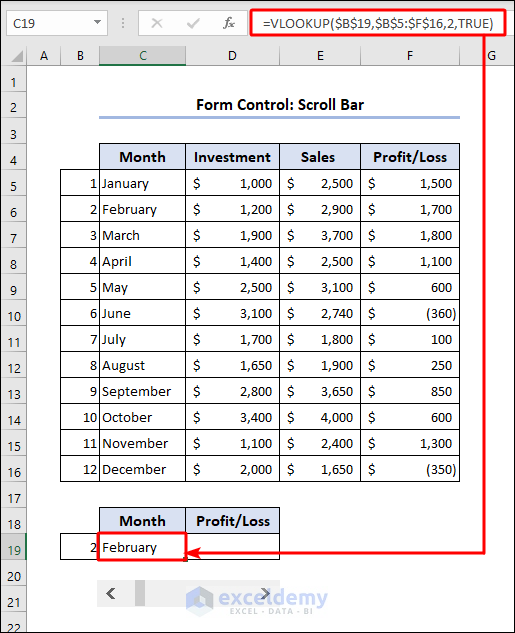

To get the Profit/Loss for the respective month in cell D19, use this formula based on the VLOOKUP function and press Enter.

=VLOOKUP($B$19,$B$5:$F$16,5,TRUE)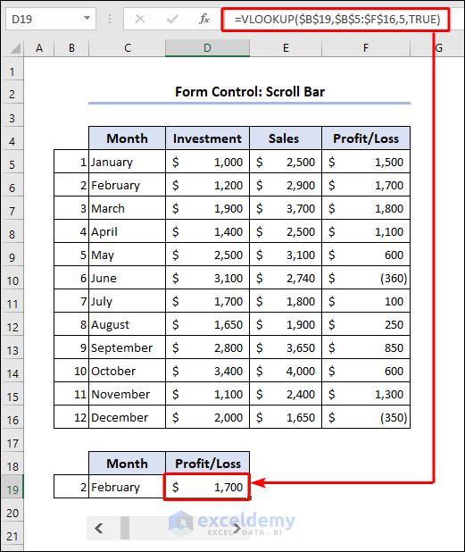

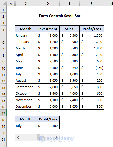
Hide the helper column B, and you will get this.

Download Practice Workbook

Download this file to practice with the article.

Excel Form Control.xlsm

Excel form Control: Knowledge Hub

How to Use Form Controls
How to Remove a Form Control
How to Create a Chart Slider
How to Make Games
Excel Checkbox
Key Differences in Excel: Form Control Vs. ActiveX Control

<< Go Back to Learn Excel

Get FREE Advanced Excel Exercises with Solutions!

SaveSavedRemoved 0

Tags: Learn Excel

Mehedi Hassan

Mehedi Hassan, having earned a BSc in Naval Architecture & Engineering from Bangladesh University of Engineering and Technology, functions as an Excel & VBA Content Developer at ExcelDemy. His deep interest in research and innovation aligns seamlessly with his fervor for Excel. In this role, Mehedi not only skillfully addresses challenging issues but also exhibits enthusiasm and expertise in gracefully navigating intricate situations, emphasizing his unwavering dedication to consistently delivering outstanding content. His interests are Advanced... Read Full Bio

We will be happy to hear your thoughts

Leave a reply Cancel reply

Submit Excel Problem