In this article, we will demonstrate how to create a Poker Machine Game in Excel. The free template of the game is downloadable at the bottom of the article. We used Microsoft Excel 365 version to create this article.
Step 1 – Forming Basic Outlines
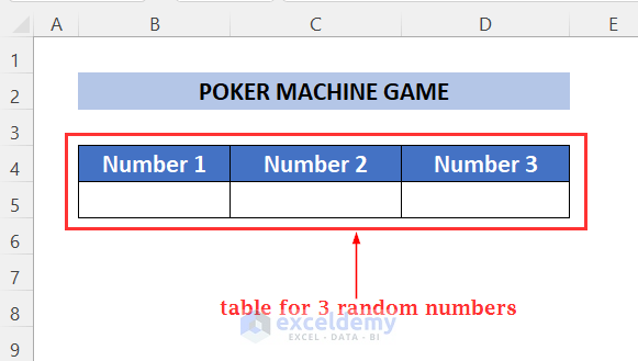
First, we will form a basic outline for entering our formulas, input values and output values.
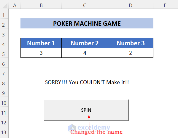
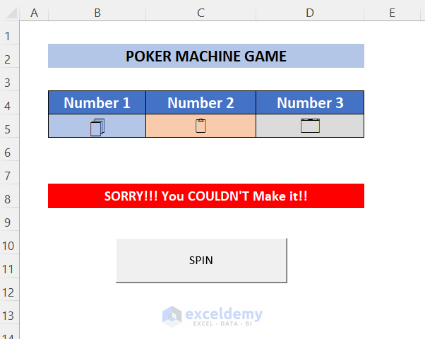
- Give a title for your game’s name, such as POKER MACHINE GAME.

- Create a table with borders in which to place 3 random numbers.
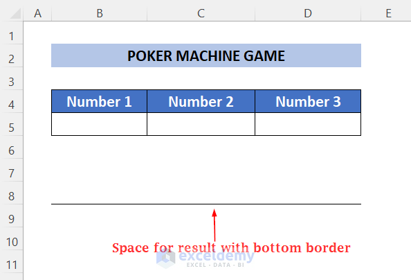
- Designate space for the output result by merging three cells, and enabling the bottom border.
Step 2 – Inserting Formulas
Now we will use the RANDBETWEEN function to generate some random numbers, and the IF and AND functions to get output results depending on these random numbers.
- Enter the following function in cell B5:
=RANDBETWEEN(1,4)1 is the start number and 4 is the end number. The function will return a value between these numbers.
- Drag the Fill Handle tool to the right until cell D5.
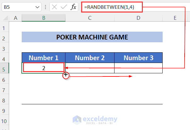
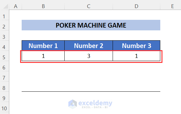
3 random numbers are generated.
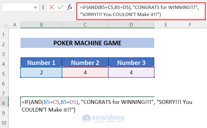
- To generate the result, use the following formula:
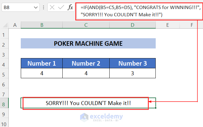
=IF(AND(B5=C5, B5=D5), "CONGRATS for WINNING!!!", "SORRY!!! You COULDN'T Make it!!")Formula Breakdown
AND(B5=C5, B5=D5) → AND will ensure that the two conditions are satisfied within this function, which returns TRUE or FALSE.
“CONGRATS for WINNING!!!” → Is the message for the logical argument TRUE.
“SORRY!!! You COULDN’T Make it!!” → Is the message returned if the argument is FALSE.
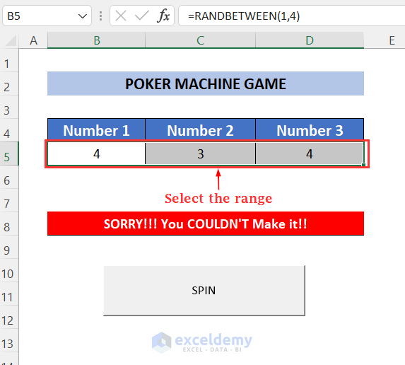
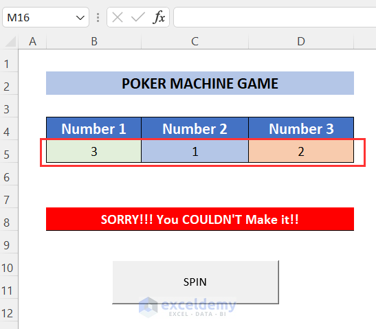
As the numbers are not matched with each other here, the message “SORRY!!! You COULDN’T Make it!!” is returned.
Step 3 – Recording Macros
Now we will record a macro to change the input numbers, and assign this macro to a button.
- Go to the Developer tab >> Insert group >> Button (Form Control).
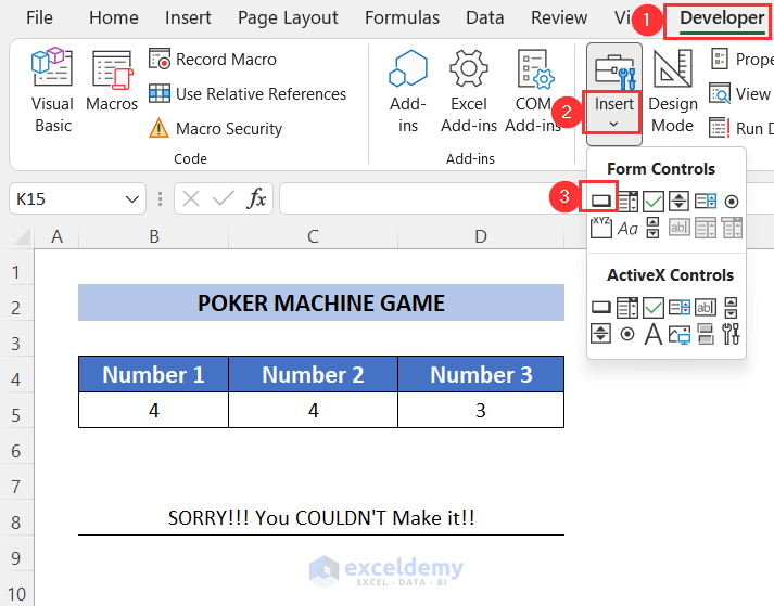
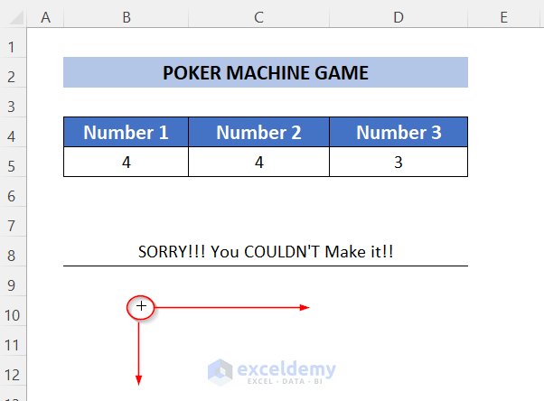
A plus (+) symbol will appear.
- Drag this symbol to the right and down.
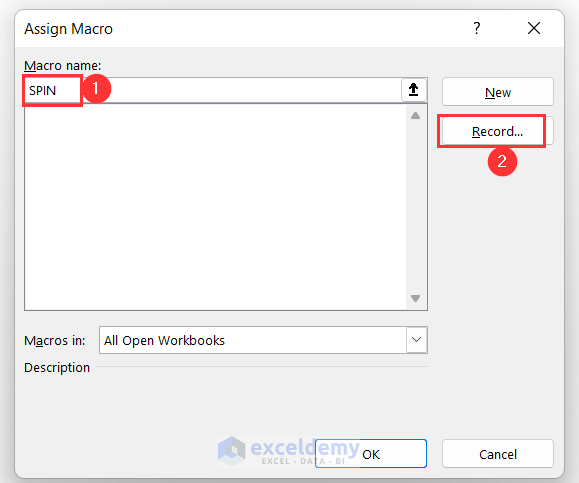
The Assign Macro wizard will open up.
- Name the macro SPIN, and click on Record.
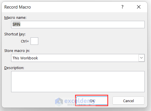
The Record Macro wizard will open.
- Click OK.
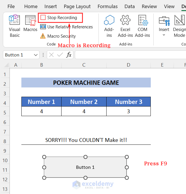
The Stop Recording option is displayed, which means our next action will be recorded as a macro.
- Press F9 to change the random numbers.
- Click on the Stop Recording button under the Developer tab.
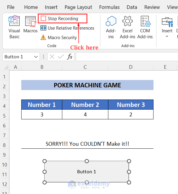
We have assigned our recorded macro to the button.
- Change the name of the button to SPIN.
Read More: How to Use Form Controls in Excel
Step 4 – Conditional Formatting of Cell with Result
Now we will change the color of the output cell depending on the cell value to make it easy to see if we won or not.
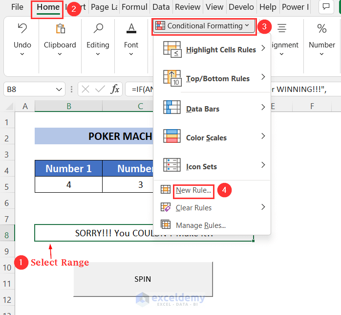
- Select the range.
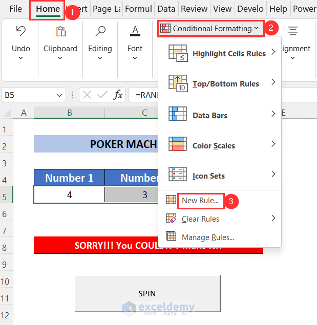
- Go to the Home tab >> Conditional Formatting group >> New Rule.
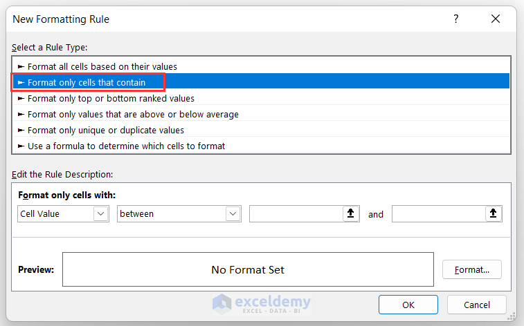
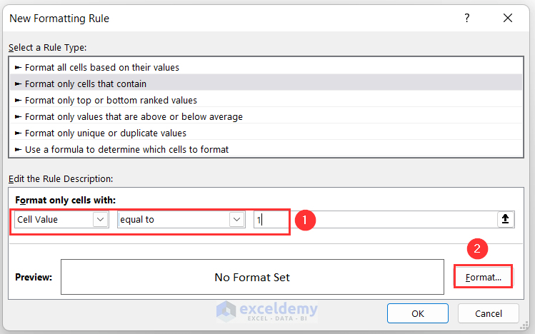
The New Formatting Rule wizard will open.
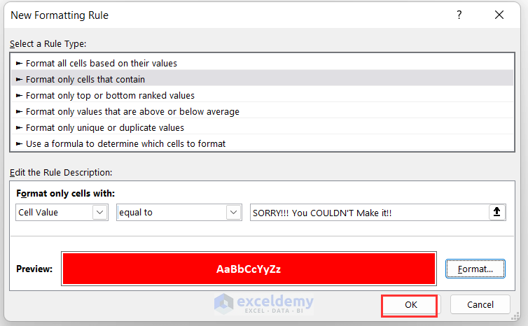
- Click on the option Format only cells that contain.
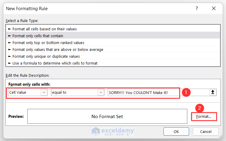
- Select Cell Value equal to SORRY!!! You COULDN’T Make it!!.
- Click on Format.
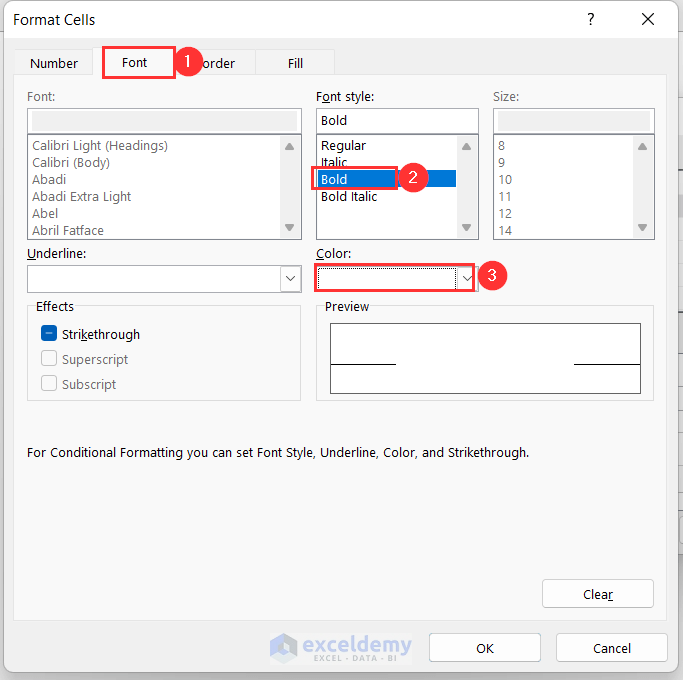
The Format Cells dialog box will appear.
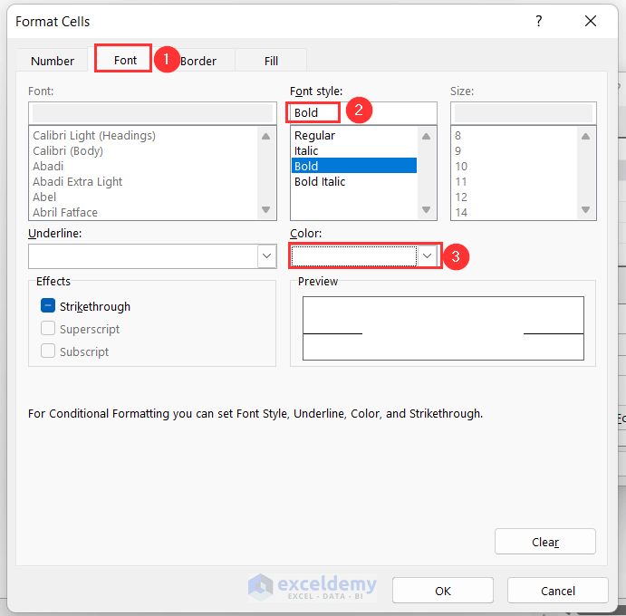
- Under the Font tab, choose the Font style as Bold, and the color as White.
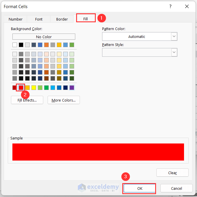
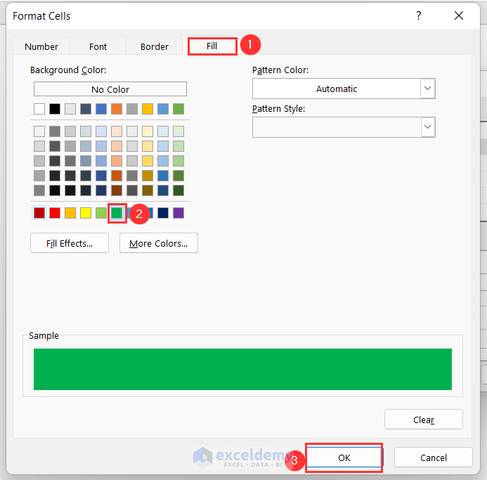
- Go to the Fill tab, choose the Background Color as Red, and click OK.
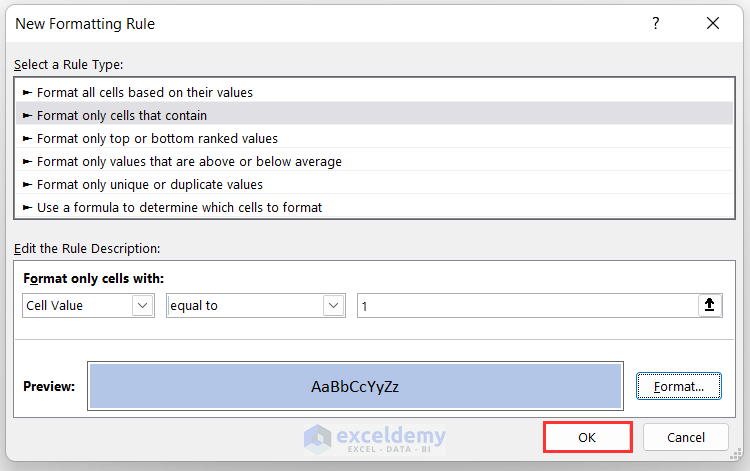
The following preview is displayed.
- Press OK.
Follow the same process for the other message:
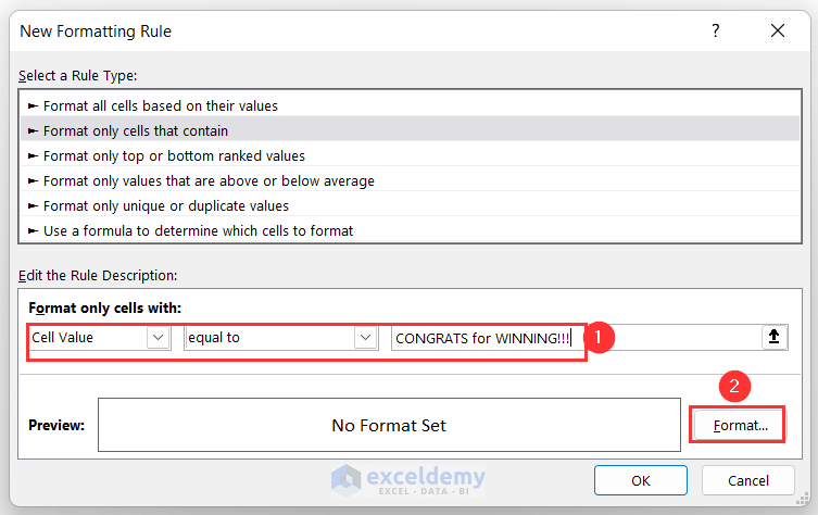
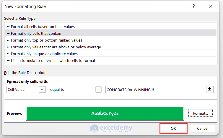
- In the New Formatting Rule wizard, click on the option Format only cells that contain.
- Put Cell Value equal to CONGRATS for WINNING!!!, and click on Format.
The Format Cells dialog box will appear.
- Under the Font tab, choose the Font style as Bold, and the Color as White.
- Go to the Fill tab, choose the Background color as Green, and click OK.
The following preview is displayed.
- Click OK.
Step 5 – Formatting Cells with Input Values
Now we will change the colors of the input cells according to their values.
- Select the range.
- Go to the Home tab >> Conditional Formatting group >> New Rule.
- In the New Formatting Rule wizard, click on the option Format only cells that contain.
- Put Cell Value equal to 1 and click on Format.
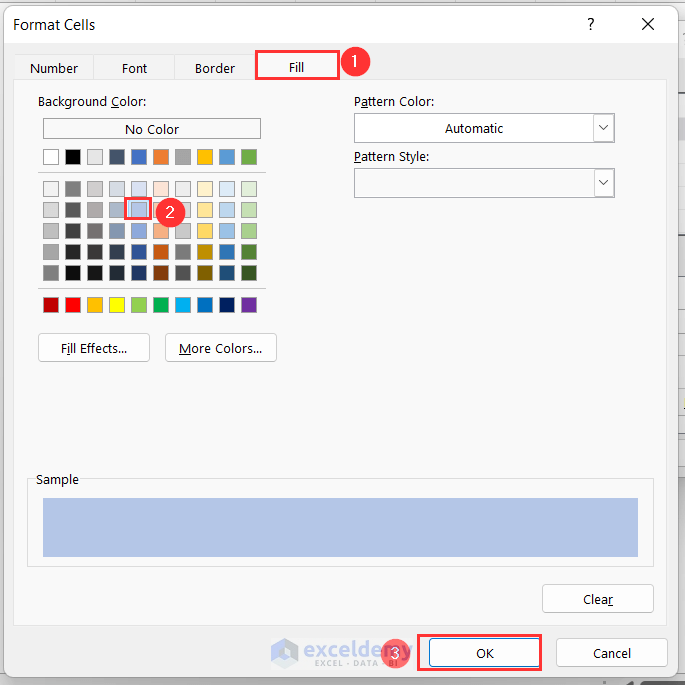
The Format Cells dialog box will appear.
- Under the Fill tab, choose the appropriate color (for example Blue, Accent 1, Lighter 60%).
- Click OK.
The following preview is displayed.
- Click OK.
- Similarly, assign different colors for other values.
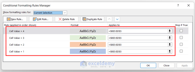
According to the conditions, the following colors will appear for their respective values.
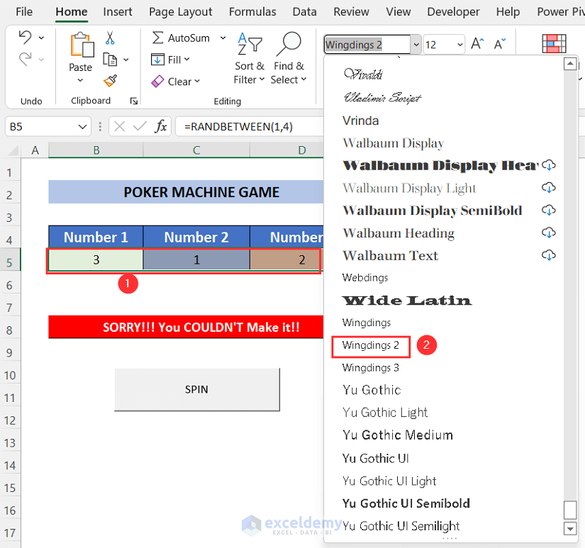
To show the numbers as symbols, which will make this game more visually appealing, we will change the font.
- After selecting the values, select the font Wingdings 2.
- Change the Font size to 16.
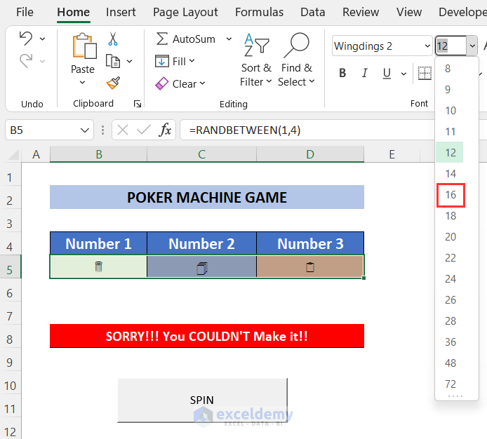
The final look of our game will be like the following:
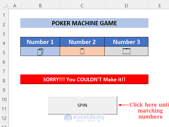
Step 6 – Play the Game!
You can now play this game by clicking on the SPIN button until the number matches.
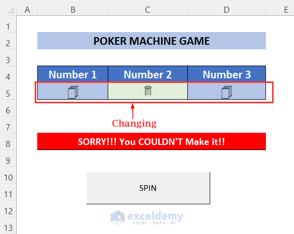
Notice the change in the numbers after pressing the button.
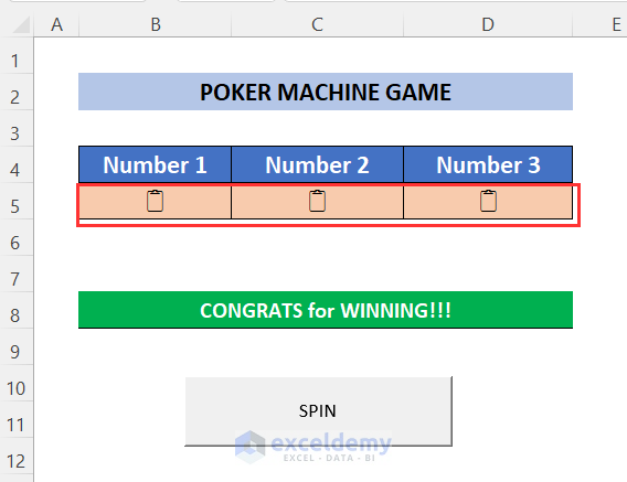
After pressing a few times, we matched the numbers and won the game.
Download Workbook
Related Articles
- How to Remove a Form Control in Excel
- How to Create Chart Slider in Excel
- Key Differences in Excel: Form Control Vs. ActiveX Control
<< Go Back to Form Control in Excel | Learn Excel
Get FREE Advanced Excel Exercises with Solutions!
