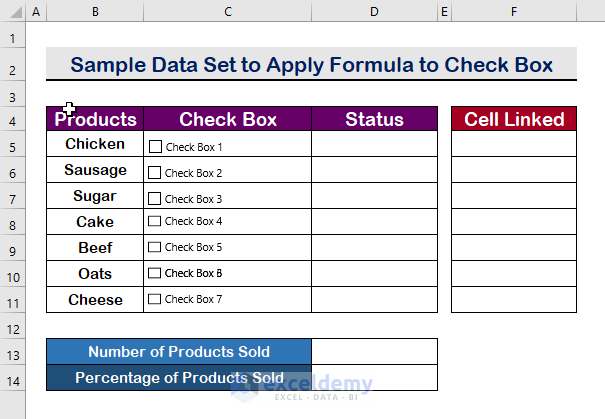
Here’s the data set we will use to insert checkboxes and apply formulas based on whether they are checked.
Method 1 – Apply Formula Based on the Cell Value If a Checkbox Is Checked
Steps:
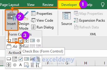
- Click on the Developer tab from the Ribbon.
- Click on Insert.
- Select Check Box (Form Control).
- Place a checkbox in a cell.
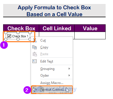
- Right-click on the checkbox.
- Select Format Control.
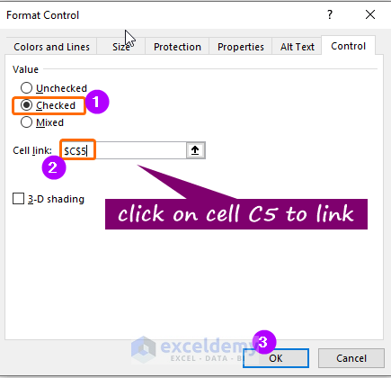
- Click on Checked.
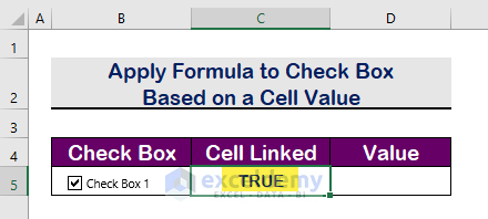
- In the Cell link box, link a cell by clicking the desired cell. We have linked cell C5 in our example.
- Press Enter.
- The cell will show TRUE when the Checkbox is checked and FALSE when the checkbox is unchecked.
- Apply the following formula in D5:
=IF(C5,"ExcelDemy", " ")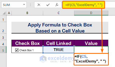
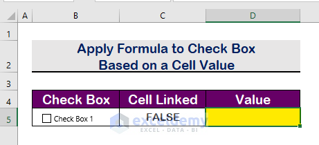
- When the Checkbox is unchecked, it returns a blank value as shown in the image below.
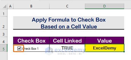
- When the Checkbox is checked, it returns the value ExcelDemy.
Notes. Sometimes, you may not have the Developer tab available if you never needed it. To activate the Developer tab:
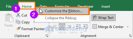
- Right-click the Home tab or any other tab from the Ribbon.
- Select Customize the Ribbon
- Check the Developer (Custom) tab.
- Click OK.
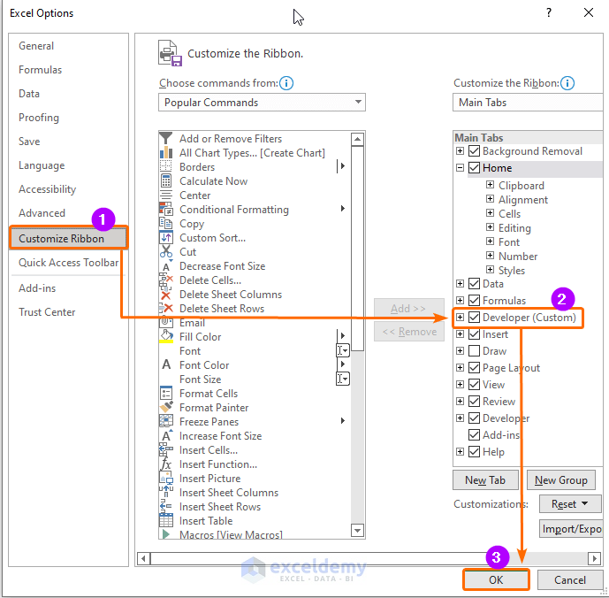
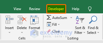
- You will see the Developer tab in the Ribbon.
Read More: What Can You Do with Cell Value If Checkbox Is Checked in Excel?
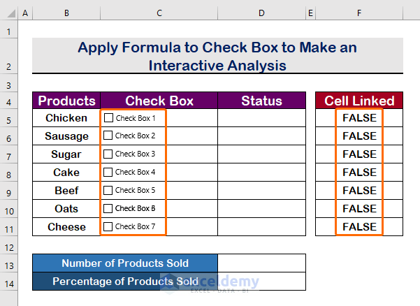
Method 2 – If a Checkbox Is Checked Then Apply Formula to Make an Interactive Analysis in Excel
Steps:
- Insert some Checkboxes in your desired cells.
- Link every Checkbox to the cells in the F column as before.
- Insert the following formula in D5:
=IF(F5,"Sold","Unsold")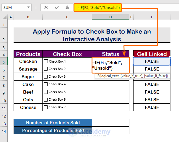
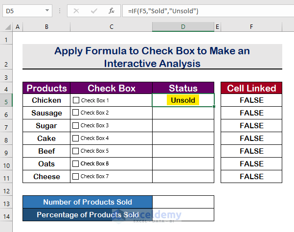
- Press Enter to see the first result.
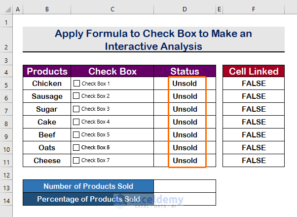
- Use AutoFill for the rest of the column.
- To count the TRUE results or the Sold result, apply the COUNTIF function with the following formula:
=COUNTIF(F5:F11,TRUE)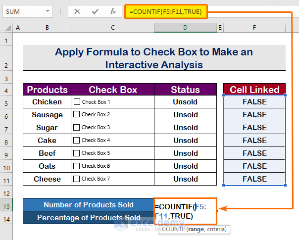
- To get the result as a percentage, divide the number of sold products by the number of total products by using the following formula.
=(D13/7)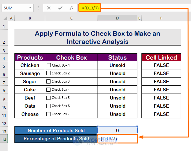
- Press Ctrl + Shift + 5 to convert the result into a percentage.
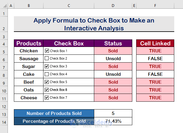
- If you check the Checkboxes, it will show the results with changes in multiple cells.
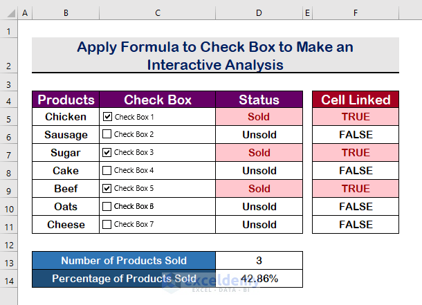
- Here’s a sample result.
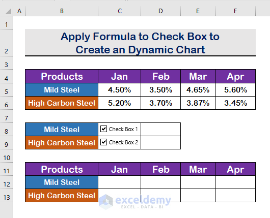
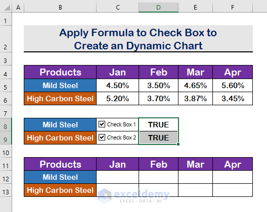
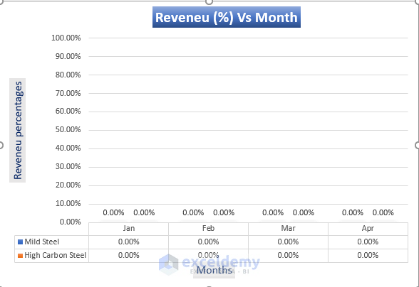
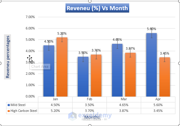
Method 3 – Create a Dynamic Chart If a Checkbox Is Checked in Excel
In the following chart, we have shown the increase in the price of Mild Steel and High Carbon Steel.
Steps:
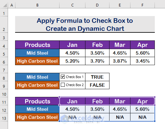
- Link cells D8 and D9 to Check Box 1 and Check Box 2.
- In cell C12, use the following formula:
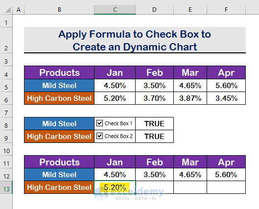
=IF($D$8,C5, "N/A")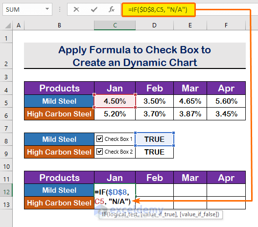
- This will show the value of cell C5 if the Checkbox is checked.
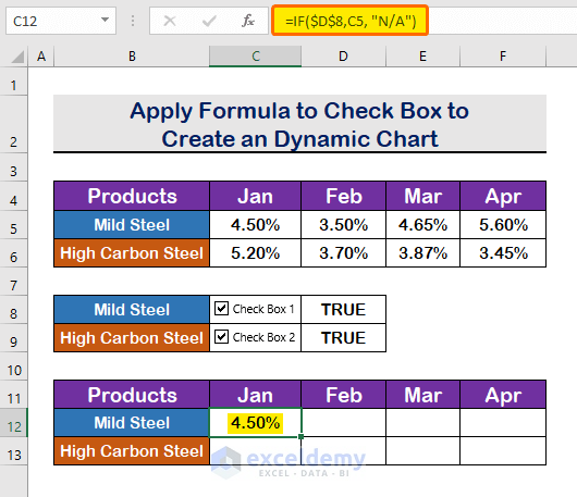
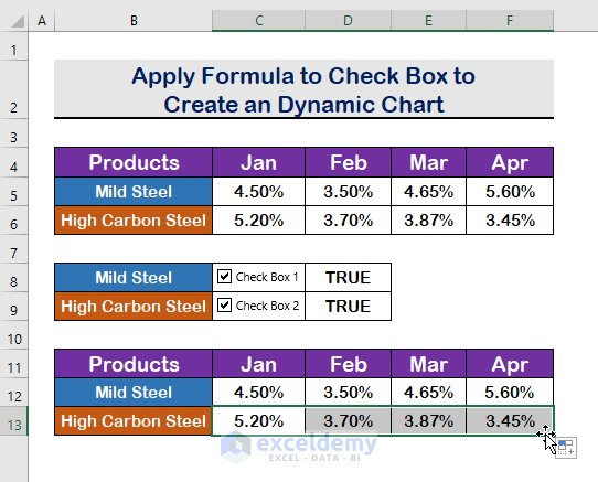
- Use the Autofill handle tool to get all the values of the range C5:F5.
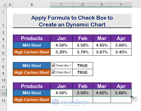
- Repeat the same procedure for High Carbon Steel. Use the following formula in the cell.
=IF($D$9,C6, "N/A")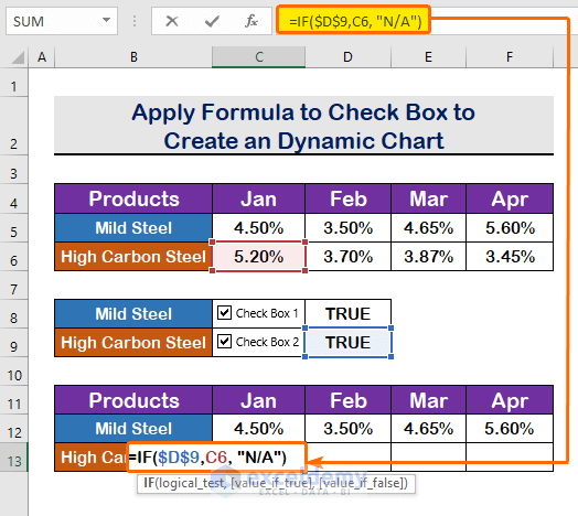
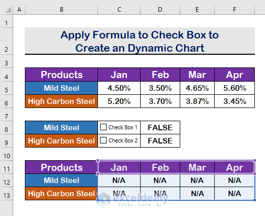
- This will show the value of cell C6 for the TRUE argument and N/A otherwise.
- Use the Autofill handle tool to fill up the other cells.
- Uncheck the box to see the changes.
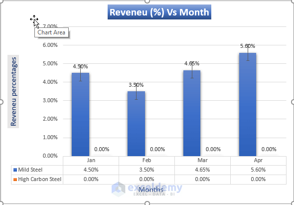
- Insert a chart for the range C12:F13.
- Check the Check Box 1.
- You will see the changes in the chart for the value of Mild steel.
- Check the Check Box 2.
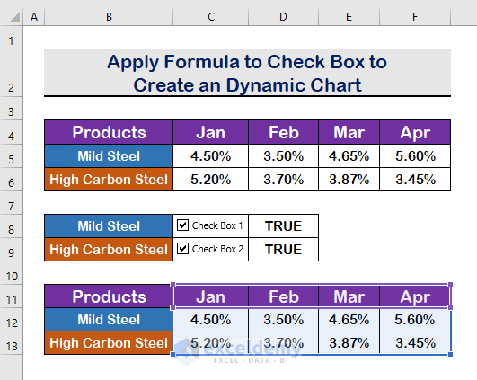
- The chart will show both the results for the Mild Steel and the High Carbon Steel.
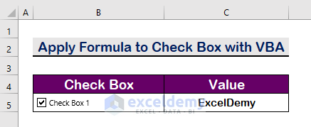
Method 4 – If a Checkbox Is Checked Then Apply a Code Based on Cell Value in Excel VBA
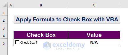
We want the value ExcelDemy to show in cell C5 when the box is checked and N/A when it remains unchecked.
Steps:
- After creating a checkbox, press Alt + F11 to open the VBA window.
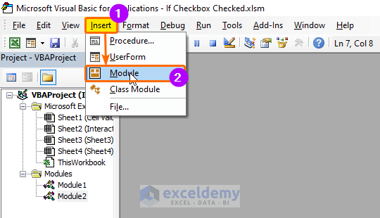
- Click on Insert.
- Select Module.
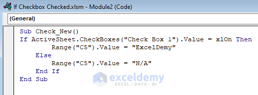
- Paste the following VBA code into the module:
Sub Check_New()
If ActiveSheet.CheckBoxes("Check Box 1").Value = xlOn Then
        Range("C5").Value = "ExcelDemy"
    Else
        Range("C5").Value = "N/A"
    End If
End Sub
- Save the program and press F5 to run it.
- Uncheck the checkbox, and you will see that the result in cell C5 is N/A.
- Check the box and you will get the result ExcelDemy as shown in the image below.
Read More: VBA to Check If CheckBox Is Checked in Excel
Download the Practice Workbook
Related Articles
<< Go Back to Excel CheckBox | Form Control in Excel | Learn Excel
Get FREE Advanced Excel Exercises with Solutions!

Bhubon,
Best examples I’ve found in my search but not getting to the answer I need.
So I have column where various checkboxes should change the date of a single cell where I am attempting to write a formula to handle the answer TRUE to change the date.
example
A27 — Expire Date 7/13/2024
A38 — Check box1 = TRUE on 2/2/2024
A27 — Expire date = TODAY() + 180 Expire date changes to 7/31/2024
A42 — check box2 = TRUE on 2/10/2024
Expire date = TODAY() + 180 Expire date expected change to 8/8/2024 but not unless changing 2/2/2024 back to FALSE answer which I don’t want to do.
This sequence continues for 8 possible iterations in a single column for each section of a project.
Tried IF(A38=TRUE,A27=TODAY()+180,IF(A42=TRUE,A27=TODAY()+180))
Or as IFS.
I would appreciate any help. Thank you sincerely.
Hello John
Thanks for your compliments! Your appreciation means a lot to us.
I have reviewed your requirements. To do so, first, you must create helper cells to store the dates associated with each checkbox when marked TRUE. Next, use the MAX function to find the latest date from these helper cells. Finally, the latest date calculates the new expiration date in A27. Please check the following:
Follow these steps:
Hopefully, these ideas will help you reach your goal. I have attached the solution workbook as well. Good luck.
DOWNLOAD SOLUTION WORKBOOK
Regards
Lutfor Rahman Shimanto
ExcelDemy