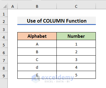
How to Convert Alphabet to Number in Excel

This is the sample dataset.

Method 1 – Converting Single Alphabet letters to Numbers in Excel

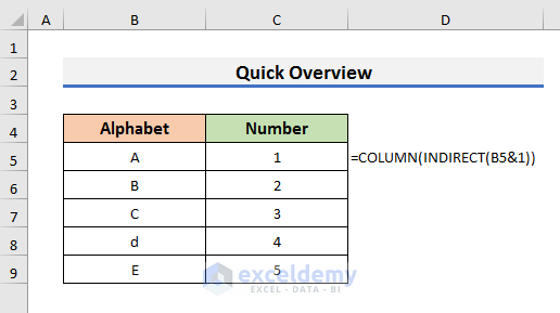
1.1 Using the COLUMN Function

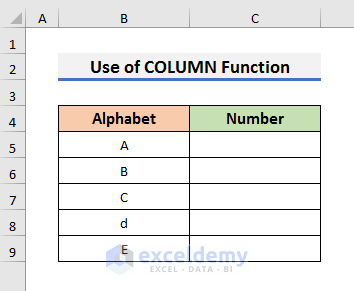
STEPS:

Select B5 and enter the formula below:

=COLUMN(INDIRECT(B5&1))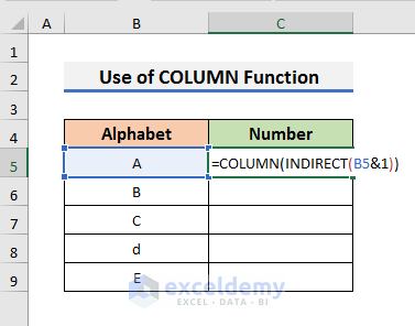

The INDIRECT function returns the reference given by a text string and the COLUMN function returns the column number of a reference. The INDIRECT(B5&1) becomes A1. Then, the formula becomes COLUMN(A1). It returns 1.

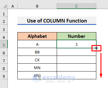
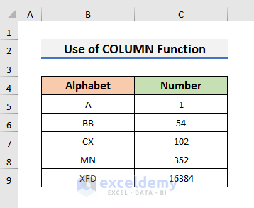
Press Enter and drag down the Fill Handle.

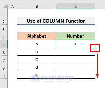
This is the output.

1.2 Applying the CODE Function

STEPS:

Enter the formula in C5:

=CODE(UPPER(B5))-64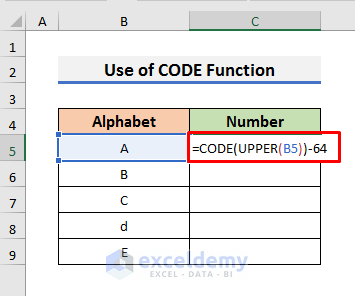

the UPPER function inside the CODE function converts the alphabet into an upper-case. The CODE function converts it into a numerical value. Here, the numerical value of A is 65. 64 is subtracted to get 1.

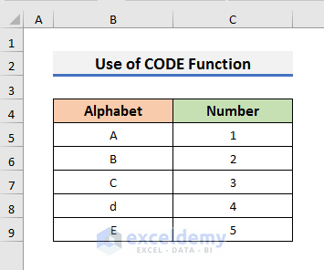
Press Enter and drag down the Fill Handle to see the result.

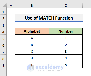
1.3 Inserting the MATCH Function

STEPS:

Select C5 and enter the formula below:

=MATCH(B5&"1",ADDRESS(1,COLUMN($1:$1),4),0)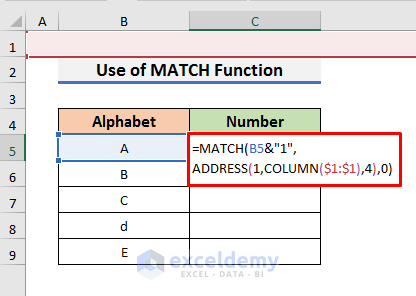

The ADDRESS function returns a relative cell reference as text and the MATCH function returns the output: 1.

Press Enter and drag the Fill Handle down.

Method 2 – Changing Multiple Alphabet letters to Numbers with the TEXTJOIN & VLOOKUP Functions

The sample dataset contains a list of alphabet letters.

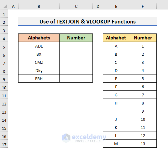
STEPS:

Select C5 and enter the formula below:

=TEXTJOIN("",1,VLOOKUP(T(IF(1,MID(B5,ROW(INDIRECT("1:"&LEN(B5))),1))),E5:F30,2,0))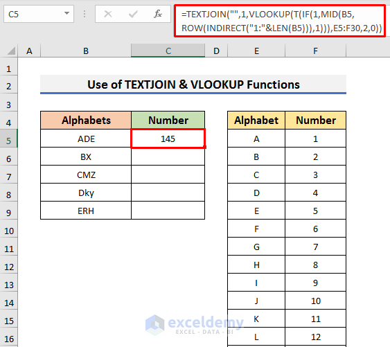

Formula Breakdown

ROW(INDIRECT(“1:”&LEN(B5))): returns the array of the row number. Here, {1,2,3}.
MID(B5,ROW(INDIRECT(“1:”&LEN(B5))),1): The MID function gives us the characters in the specified position of the given string. The output is {A,D,E}.
VLOOKUP(T(IF(1,MID(B5,ROW(INDIRECT(“1:”&LEN(B5))),1))),E5:F30,2,0): The VLOOKUP function looks for the corresponding numbers in the array {A,D,E} in E5:F30.
TEXTJOIN(“”,1,VLOOKUP(T(IF(1,MID(B5,ROW(INDIRECT(“1:”&LEN(B5))),1))),E5:F30,2,0)): The TEXTJOIN function joins the numbers and returns the output 145.

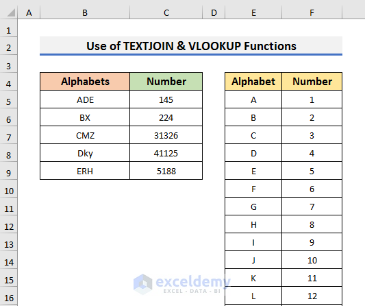
Press Enter.
Drag down the Fill Handle to see the result.

Method 3 – Inserting the SUBSTITUTE Function to Transform Specific Alphabet letters to Numbers

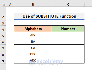
STEPS:

Enter the formula below in C5:

=SUBSTITUTE(SUBSTITUTE(SUBSTITUTE(SUBSTITUTE(B5,"A",1),"B",2),"C",3),"D",4)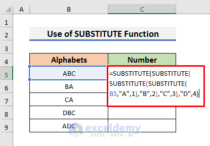

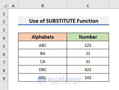
The formula substitutes A with 1, B with 2, C with 3, and D with 4. The output of ABC is 123.

Press Enter.
Drag the Fill Handle down to see the result.

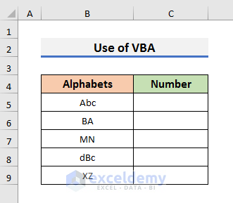
Method 4 – Applying a VBA to Convert Letters to Numbers in Excel

This is the sample dataset.

STEPS:

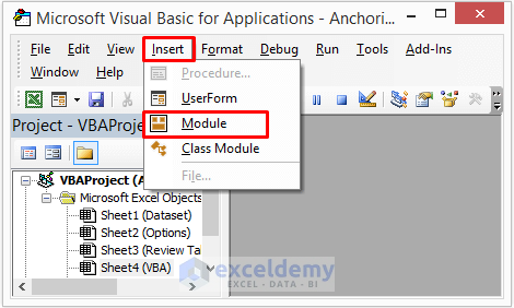
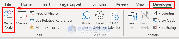
Go to the Developer tab and select Visual Basic.The Visual Basic window opens.

In the Visual Basic window, select Insert >> Module. The Module window opens.

Enter the code below in the Module:

Option Explicit
Function AlphabetToNumber(ByVal sSource As String) As String
Dim x As Integer
Dim sResult As String
For x = 1 To Len(sSource)
    Select Case Asc(Mid(sSource, x, 1))
        Case 65 To 90:
            sResult = sResult & Asc(Mid(sSource, x, 1)) - 64
        Case Else
            sResult = sResult & Mid(sSource, x, 1)
    End Select
Next
AlphabetToNumber = sResult
End Function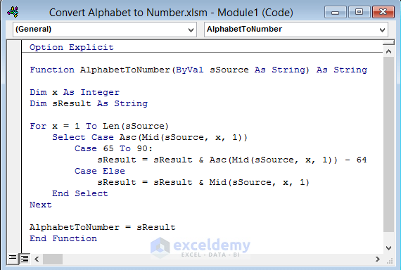

This VBA code creates a function that converts the alphabet to numbers. To apply the function for lower and upper cases, use the UPPER function inside the AlphabetToNumber function.

Press Ctrl + S to save the code.
Select C5 and enter the formula below:

=AlphabetToNumber(UPPER(B5))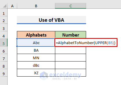

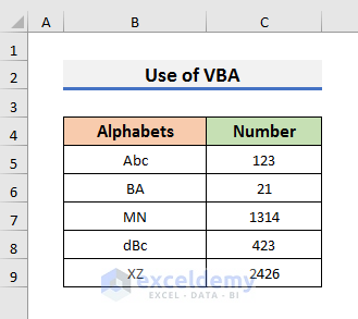
Drag the Fill Handle down to see the result.

How to Convert Alphabet to Number in a Column in Excel.

1. Converting Alphabet to Number Using Excel COLUMN Function

STEPS:

Select Cell C5 and enter the formula below:

=COLUMN(INDIRECT(B5&1))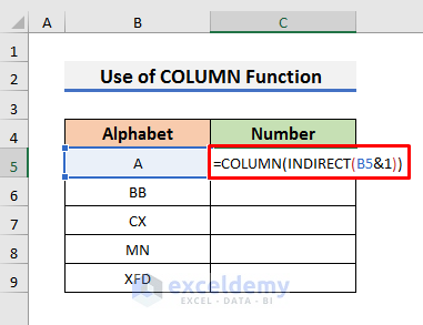

The INDIRECT(B5&1) becomes A1. The formula becomes COLUMN(A1) and returns 1.

Press Enter and drag the Fill Handle down.

You will see the column numbers.

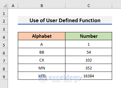
2. Applying the User Defined Function to Change Column Letter to Number in Excel

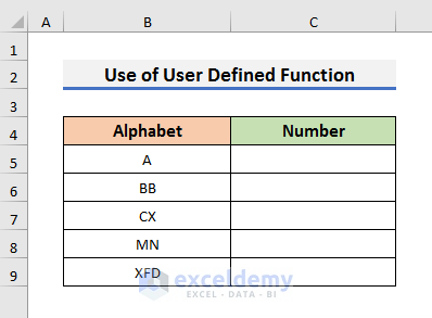
STEPS:

Go to the Developer tab and select Visual Basic to open the Visual Basic window.

Select Insert >> Module. The Module window opens.

Enter the code below in the Module window:

Public Function ColNumber(cletter As String) As Long
  ColNumber = Columns(cletter).Column
End Function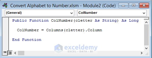

ColNumber returns the column number and cletter is the argument of the function (enter the cell that contains the column letters).

Press Ctrl + S to save.
Select C5 and enter the formula below:

=ColNumber(B5)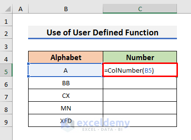

Press Enter and drag the Fill Handle down.

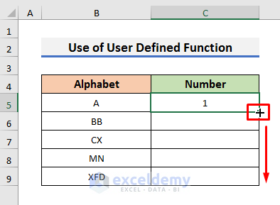
This is the output.

Download Practice Workbook

Convert Alphabet to Number.xlsm

<< Go Back to Convert Text to Number in Excel | Learn Excel

Get FREE Advanced Excel Exercises with Solutions!

Option Explicit Function AlphabetToNumber(ByVal sSource As String) As String Dim x As Integer Dim sResult As String For x = 1 To Len(sSource) Select Case Asc(Mid(sSource, x, 1)) Case 65 To 90: sResult = sResult & Format(Asc(Mid(sSource, x, 1)) - 64, "00") Case Else sResult = sResult & Mid(sSource, x, 1) End Select Next AlphabetToNumber = sResult End Function

Function ConvertNumbersToLetters(inputStr As String) As String Dim numArray() As String Dim resultArray() As String Dim i As Integer Dim currentNum As String Dim convertedNum As String numArray = Split(inputStr, ",") ReDim resultArray(LBound(numArray) To UBound(numArray)) For i = LBound(numArray) To UBound(numArray) currentNum = Trim(numArray(i)) convertedNum = "" Dim j As Integer Dim currentChar As String For j = 1 To Len(currentNum) currentChar = Mid(currentNum, j, 1) Select Case currentChar Case "1" convertedNum = convertedNum & "A" Case "2" convertedNum = convertedNum & "B" Case "3" convertedNum = convertedNum & "C" Case "4" convertedNum = convertedNum & "D" Case "5" convertedNum = convertedNum & "E" Case "6" convertedNum = convertedNum & "F" Case "7" convertedNum = convertedNum & "G" Case "8" convertedNum = convertedNum & "H" Case "9" convertedNum = convertedNum & "I" Case "0" convertedNum = convertedNum & "O" Case Else convertedNum = convertedNum & currentChar End Select Next j resultArray(i) = convertedNum Next i ConvertNumbersToLetters = Join(resultArray, ", ") End Function

8 Comments

harman Apr 25, 2024 at 3:48 PM

I want to convert e.g
AA=0101
GF=0706
WA=2301
Still in search of this formula in excel… I’m very close to it like
AA=11
GF=76
WA=231
But we want 0 as leading above example when we convert A to I in number.
- Reply
  Lutfor Rahman Shimanto Apr 25, 2024 at 5:18 PM
  Hello Harman
  
  Thanks for visiting our blog and sharing your query. You want 0 as leading when returning a number against a character. Don’t worry! I have come up with two solutions:
  
  Use of TEXTJOIN, TEXT & VLOOKUP Functions
  Select an empty cell.
  
  Insert the following formula: =TEXTJOIN("", 1, TEXT(VLOOKUP((IF(1, MID(B5, ROW(INDIRECT("1:" & LEN(B5))), 1))), $E$5:$F$30, 2, 0), "00"))
  
  Drag the Fill Handle icon to copy the formula down.
  Use of VBA User-Defined Function
  Go to Developer, followed by Visual Basic.
  
  Click on Insert followed by Module.
  
  Insert the following code in the module and save it:
  Option Explicit Function AlphabetToNumber(ByVal sSource As String) As String Dim x As Integer Dim sResult As String For x = 1 To Len(sSource) Select Case Asc(Mid(sSource, x, 1)) Case 65 To 90: sResult = sResult & Format(Asc(Mid(sSource, x, 1)) - 64, "00") Case Else sResult = sResult & Mid(sSource, x, 1) End Select Next AlphabetToNumber = sResult End Function
  
  Return to the sheet and select an empty cell.
  
  Insert the following formula: =AlphabetToNumber(UPPER(B5))
  
  Hit Enter to see an output like the following GIF:
  I hope the formulas and VBA code will fulfil your goal. I have attached the solution workbook; good luck.
  
  DOWNLOAD SOLUTION WORKBOOK
  
  Regards
  Lutfor Rahman Shimanto
  Excel & VBA Developer
  ExcelDemy
harman May 6, 2024 at 12:08 PM

Thanks its working.
- Reply
  Lutfor Rahman Shimanto May 6, 2024 at 12:32 PM
  
  Dear Harman
  Thanks for thanking me. You are most welcome. We are glad the solution worked perfectly.
  
  Regards
  ExcelDemy

Rahul Dixit May 29, 2024 at 7:14 PM

I want to convert
1 = A
2 = B
3 = C
4 = D
5 = E
6 = F
7 = G
8 = H
9 = I
0 = O

and also wants to join them e.g. if I enter 45, 23, 67 then output should be DE, BC, FG respectively.

Lutfor Rahman Shimanto May 30, 2024 at 9:48 AM

Hello Rahul Dixit

Thanks for visiting our blog and sharing such an exciting problem! I have reviewed your problem and come up with an Excel VBA User-defined function. Please check the following:

Excel VBA Code:

Hopefully, you have found the solution you were looking for. I have attached the solution workbook as well; good luck.

DOWNLOAD SOLUTION WORKBOOK

Regards
Lutfor Rahman Shimanto
Excel & VBA Developer
ExcelDemy

SUMMERTIME SAGA APK Dec 8, 2024 at 12:46 PM

Great post! I never knew there were so many methods to convert letters to numbers in Excel. The step-by-step instructions were super helpful. Can’t wait to try them out in my next project!
- Reply
  Shamima Sultana Dec 9, 2024 at 10:46 AM
  
  Hello,
  
  You are most welcome. Thanks for your feedback and appreciation. Glad to hear that our step-by-step guide is super helpful to you.
  
  Regards
  ExcelDemy

How to Convert Alphabet to Number in Excel – 4 Easy Methods

Method 1 – Converting Single Alphabet letters to Numbers in Excel

1.1 Using the COLUMN Function

1.2 Applying the CODE Function

1.3 Inserting the MATCH Function

Method 2 – Changing Multiple Alphabet letters to Numbers with the TEXTJOIN & VLOOKUP Functions

Method 3 – Inserting the SUBSTITUTE Function to Transform Specific Alphabet letters to Numbers

Method 4 – Applying a VBA to Convert Letters to Numbers in Excel

How to Convert Alphabet to Number in a Column in Excel.

1. Converting Alphabet to Number Using Excel COLUMN Function

2. Applying the User Defined Function to Change Column Letter to Number in Excel

Related Articles

Leave a reply Cancel reply