If you are looking for simple ways to know how Excel formulas convert Text to Number, this article will serve the purpose.
While working with data in Excel, we often encounter some data that are numbers but are mistakenly stored as texts. To get rid of this silly mistake, in Excel we can easily convert text to number using Excel formulas by following some simple methods.
So, let’s start with this article and learn all the steps on how Excel formulas convert text to number.
How Are Numbers Indicated as Text in Excel?
Do you want to know how to tell if a number is entered as text in Excel?
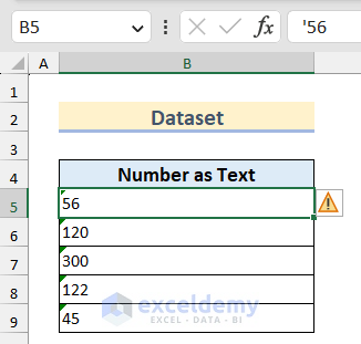
In Excel, numbers are by default entered as right aligned and text is left aligned. If you notice that your data is left aligned, then the number must be in Text format.
Another way to check is to see if there is any green flag at the top left corner of your cell. If you select the cell an error checker will appear with a message as Number Stored as Text.
Why Is Converting Text to Number Impactful in Excel?
There are a number of ways a number can be stored as text. For example, having a leading apostrophe or storing the numbers while text format is applied to the cell, etc. can be the cause of storing numbers in text format. When a number is stored in text format, we can’t do any mathematical operation or apply any formula with this data. Which is a major drawback. So, it is crucial to convert text to numbers in Excel.
How Excel Formulas Convert Text to Number: 3 Easy Ways
In this article, we are going to learn 3 easy methods of how Excel formulas convert text to number.
We have used Microsoft Excel 365 version for this article, you can use any other version according to your convenience.
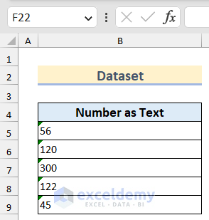
In the following dataset, we have 5 numbers that are mistakenly stored in text format. We will convert them into number format.
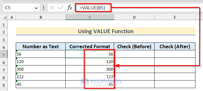
1. Using VALUE Function to Convert Text to Numbers in Excel Formula
By using the VALUE function we can easily convert text to numbers. If a text string represents a number, then the VALUE function will convert the text string into that number. Let’s follow the steps outlined below.
- Insert the following formula in cell C5.
=VALUE(B5)- Press Enter and use Excel’s Fill Handle tool to get the rest of the data like the following picture.
How to Check If Value Is Number or Not
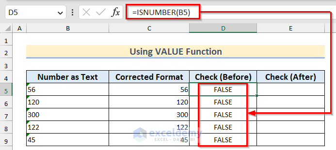
At this stage, we will check whether the texts are converted to numbers or not. To do this we will use the ISNUMBER function. If the content of a cell is a number then the ISNUMBER function will return TRUE, otherwise, it will return FALSE.
- Select cell D5 and Insert the following formula.
=ISNUMBER(B5)- Press Enter and use Excel’s Fill Handle tool to get the rest of the data like the following picture.
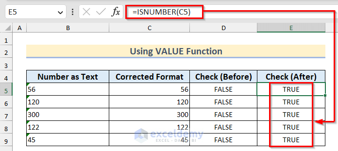
- After that, select cell E5 and Insert the following formula.
=ISNUMBER(C5)- Press Enter and use Excel’s Fill Handle tool to get the rest of the data like the following picture.
Read More: How to Fix All Number Stored as Text in Excel
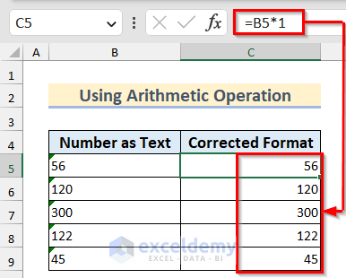
2. Convert Text to Number in Excel Using Arithmetic Operation in Formula
Multiplying by 1 is one of the most popular methods to convert text to number. Let’s see the steps mentioned below.
- Select Cell C5 and insert the following formula.
=B5*1- Press Enter and then drag down the Fill Handle tool to copy the formula to the rest of the cells.
- Thus, you can convert text values to numbers in Excel.

3. Convert Text with Space to Numbers Using VALUE, TRIM and CLEAN Functions in Excel
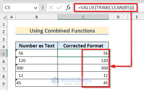
Suppose you have extra spaces and non-printing characters in your dataset. You want to convert text values to numbers and remove those extra spaces and non-printing characters. You can use the VALUE, TRIM and CLEAN functions to do that.
Here in Cell C5, we will see that the CLEAN function will remove extra spaces and non-printing characters of Cell B5. Then the TRIM function will remove any leading or trailing spaces and the VALUE function will convert text to number.
- Insert the following formula in cell C5.
=VALUE(TRIM(CLEAN(B5)))- Press Enter and use Excel’s Fill Handle tool to get the rest of the data like the following picture.
How to Convert Text to Number Without Using Formulas in Excel
You can convert text to numbers in different ways without using any formulas in Excel. Here, you will find some of those methods below.
1. Use Text to Columns Option to Convert Text to Number in Excel
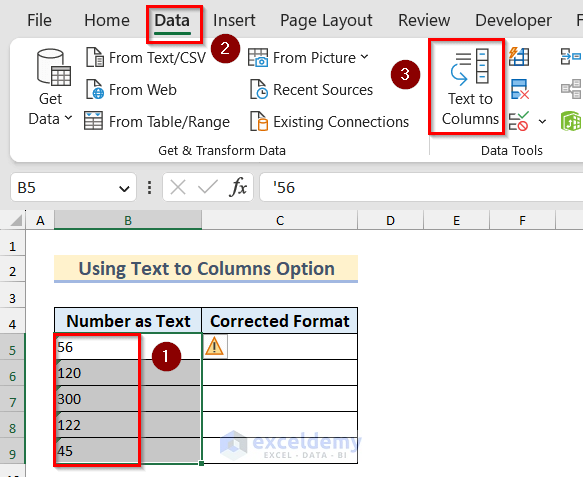
In this section of the article, we will learn to use the Text to Column feature of Excel to convert text to number. Let’s follow the steps mentioned below.
- Select the column of Number as Text.
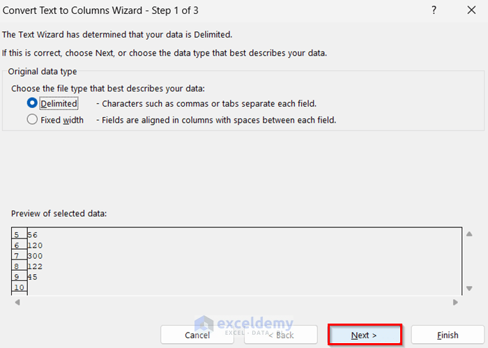
- After that, go to the Data tab >> Text to Columns option.
- A dialogue box will open on your screen like the following picture, and click Next from the dialogue box.
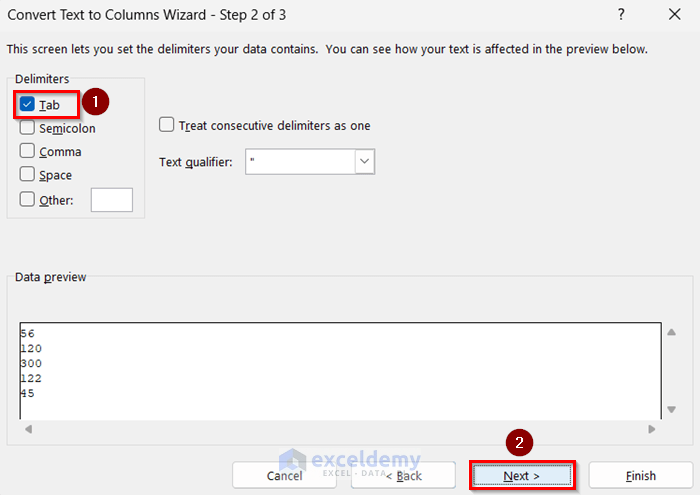
- Check the box of Tab as marked in the following image and click Next.
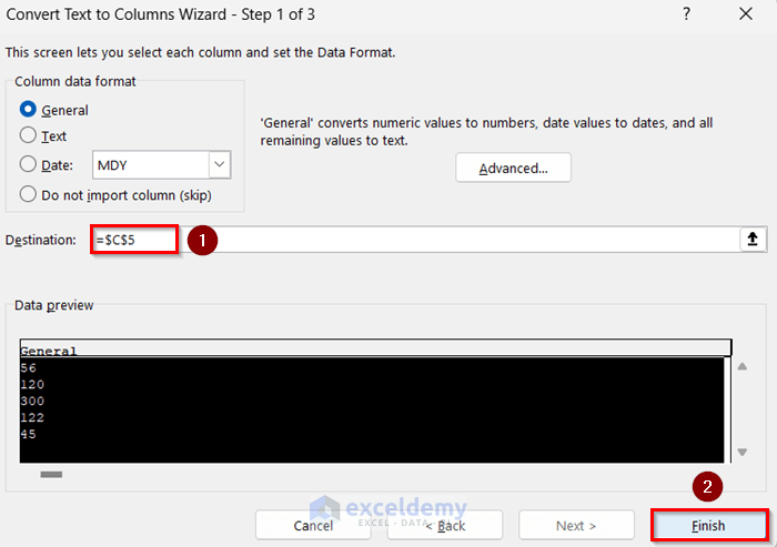
- Insert your destination cell. In this case, we have selected cell C5 and clicked on OK.
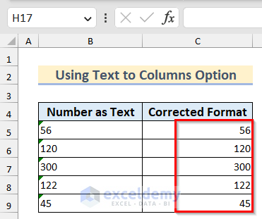
- You will be able to see the following image on your screen.
2. Apply Error Checking Button to Change Text to Number
Using the Error Checking Button is the simplest way to convert text to number. Let’s learn the steps mentioned below to do this.
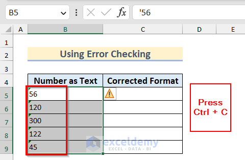
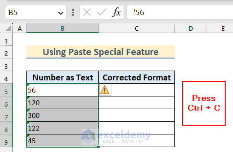
- Firstly, select the column of Number as Text and press Ctrl+C.
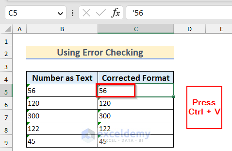
- Click on cell C5 and press CTRL+V. You will get the following table on your worksheet.
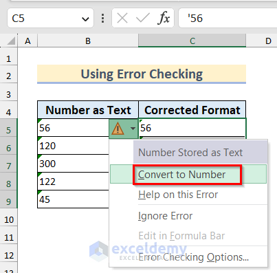
- Now, select cell range C5:C9. Click on the error icon as marked in the following picture.

- Select Convert to Number from the drop-down.
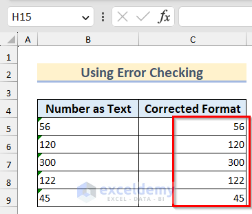
- Your data will be converted to a number format like the following image.
Read More: How to Fix Convert to Number Error in Excel
3. Convert Text into Number by Changing Number Format in Excel
You can change the Number format of a cell to convert text to number in Excel. Here are the steps to do that.
- Select Cell B5. Go to the Home tab >> select Number from Number group.
- Double-click on the cell to go to Enter mood and then press Enter.
- Thus, you can convert text to number changing Number format in Excel.
4. Change Text to Number with Paste Special Feature
You can also use the Paste Special feature to change the text to number in Excel. Here are the steps to do that.
- Select the column of Number as Text and press Ctrl + C.
- Then, select Cell C5 and press Ctrl + Alt + V to open the Paste Special box.
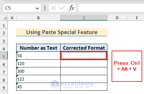
- Now, select Values from the Paste options and Add from the Operation options. After that, click on OK.

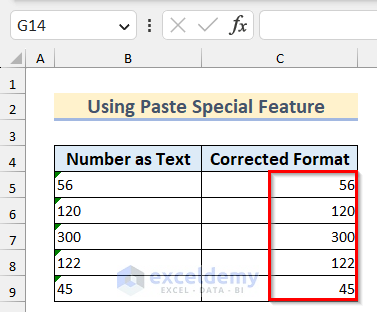
- Thus, it will copy only the values from your selected cell range.
Read More: How to Convert Green Triangle to Number in Excel
5. Use Power Pivot Feature to Convert Text to Number in Excel
We can convert text to numbers by using Power Pivot also. Let’s learn the following steps to do this in Excel.
Step 01: Enabling Power Pivot Option
If you do not have the Power Pivot option enabled in your Excel workbook follow the steps given below to do that.
- Go to the File tab.

- Select the Options tab.

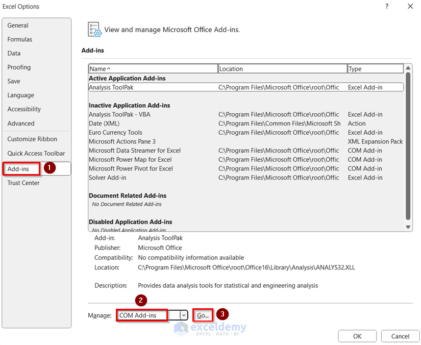
- An Excel Options dialogue box will open like the following image. Go to the Add-ins tab.
- Select COM Add-ins from the Manage drop-down options. Then, click on Go.
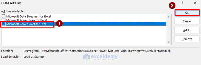
At this stage, another dialogue box will open named COM Add-ins like the following image.
- Check the box of Microsoft Office PowerPivot for Excel 2013 and click OK.
Step 02: Using Power Pivot
Now, go through the steps given below to use Power Pivot to convert text to number in Excel.
- Go to the Power Pivot tab. Now, select the dataset and click on Manage.
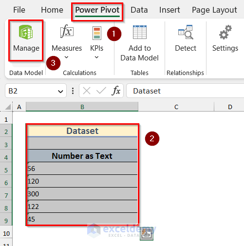
- After that, you will see the following Power Pivot box on your screen.
- Click on the cell below Add Column and insert the following formula there.
=VALUE(PastedTable[Number as Text])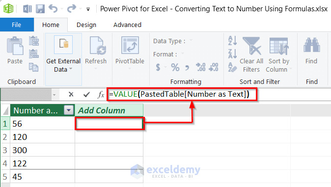
Note: To insert this formula, first, type in =VALUE(. Then double-click on the Number as Text cell. Then close parenthesis.
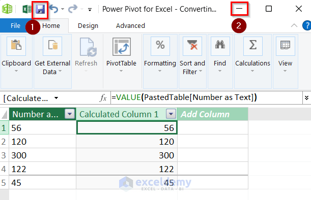
- After entering the formula, you will see the following output on your worksheet.
- Click on Save as shown in the image given below and then click on Minimize.
Step 03: Inserting Pivot Table
Finally, to show the results in your Excel worksheet go through the steps given below.
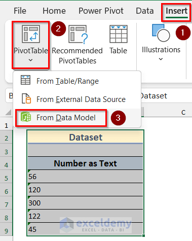
- Go to the Insert tab >> Pivot Table drop-down >> From Data Model option.
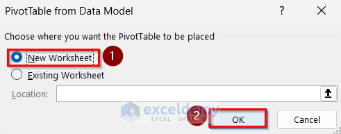
- After that, a dialogue box will open. Select New Worksheet and click OK in the dialogue box like the following image.
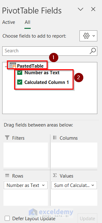
Another dialogue box named Pivot Table Fields will open on your worksheet.
- Click on PastedTable. Check the boxes of Number as Text and Calculated Column 1.
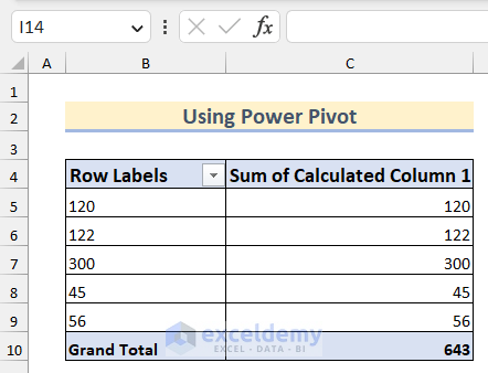
- Thus, you will have the following table on your worksheet.
Practice Section
For doing practice, we have provided a practice section in each worksheet on the right side. Please do it by yourself.
Download Practice Workbook
Conclusion
Finally, we have to the very end of the article. I truly hope that this article was able to guide you to learn the methods of how excel formulas convert text to number. Please feel free to leave a comment if you have any queries or recommendations for improving the article’s quality. Happy learning!
Related Articles
- How to Convert Alphabet to Number in Excel
- How to Convert Entire Column to Number in Excel
- How to Bulk Convert Text to Number in Excel
- How to Convert Text with Spaces to Numbers in Excel
<< Go Back to Convert Text to Number in Excel | Learn Excel
Get FREE Advanced Excel Exercises with Solutions!
