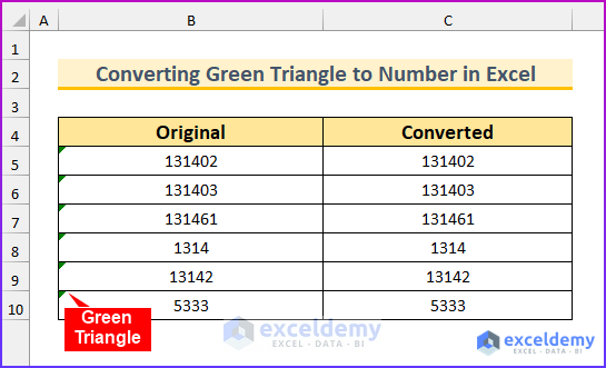
A green triangle will appear in the top-left corner of the cell when Excel detects an error in any cell. In the case of a number, this appears when that number is formatted as text. In this article, we will show you six quick methods to convert the green triangle to a number in Excel.
How to Convert Green Triangle to Number in Excel: 6 Ways
There will be six easy approaches to convert a green triangle to a number in Excel. Firstly, we will use the Convert to Number feature. Secondly, we will utilize the Paste Special option. Thirdly, we will use the Text to Column feature. Following that, we will apply the VALUE function. After that, we will use a mathematical operator. Lastly, we will employ Power Query to achieve the objective of this article. Additionally, you can see a quick view of the output of this article from the image below.
1. Using Convert to Number Option
When a cell with a green triangle is clicked, an error message is shown. In the case of the number formatted as text, this message will be shown upon hovering over the error sign: “the number in this cell is formatted as text or preceded by an apostrophe.” We can click on that error sign and select the Convert to Number option to fulfill the objective of this article.
Steps:
- Firstly, copy the values from the range B5:B10 to the range C5:C10. We are doing this for better visualization, you can replace the values.

- After that, select the entire column values.
- Then, a yellow warning sign will pop up, and click on that.
- Finally, select the Convert to Number option from that list. The following animated image shows you the process.
Read More: Excel Convert to Number Entire Column
2. Utilizing Paste Special Feature to Convert Green Triangle to Number
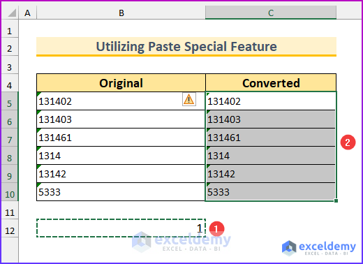
In order to turn the green triangle into a number, we will make use of the Paste Special feature. We will type 1 or 0 anywhere in the sheet, then using a keyboard shortcut, we will bring up the Paste Special dialog box. However, a copied value from an empty cell will work just fine to use this feature. Finally, we will change two settings to achieve the goal of this article.
Steps:
- To begin with, copy 1 which is in cell B12.
- Then, select the cell range C5:10 and press Ctrl+Alt+V.
- So, the Paste Special dialog box will appear.
- Then, select Values and Multiply from the Paste and the Operation sections respectively.
- Lastly, press OK.

- Thus, this will convert the green triangle to a number.

Read More: How to Convert Text with Spaces to Number in Excel
3. Using Text to Column Wizard
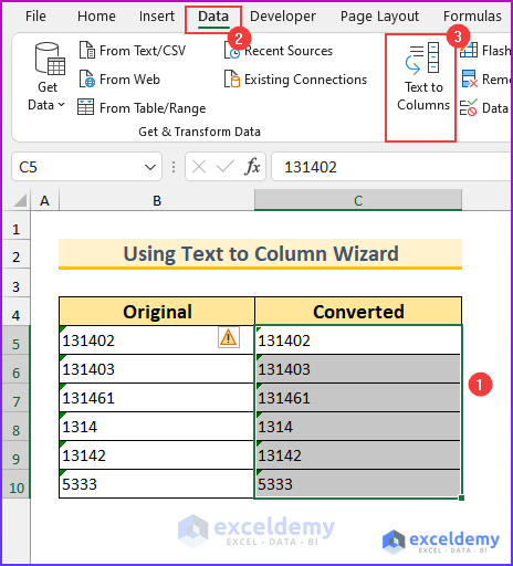
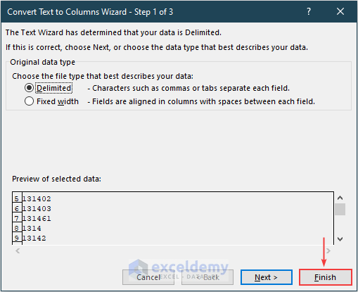
In this third method, we will use the Text to Column wizard. This feature is useful for converting the green triangle to a number in Excel. Remember, this wizard is available only in Excel 2013 and later.
Steps:
- Firstly, select the cell range C5:C10.
- Secondly, from the Data tab, select Text to Columns.
- Therefore, a dialog box will appear.
- We do not need to change anything and just press Finish.
- In conclusion, this will be the completion of third method to convert a green triangle to a number in Excel.

4. Applying VALUE Function to Convert Green Triangle to Number
In this section, we will apply the VALUE function to convert a green triangle to a number. Then, we will use the Fill Handle to apply that formula to the rest of the cells. This will AutoFill the formula in Excel to convert all the green triangles to number format.
Steps:
- To begin with, type the following formula in cell C5.
=VALUE(B5)

- Then, press Enter, and using the Fill Handle, insert the formula into the rest of the cells.

5. Using Mathematical Operator
We will use a mathematical operator in this section to convert a green triangle to a number. There are mainly four mathematical operators: addition, subtraction, multiplication, and division. If we use this with a number (formatted as text), then that pseudo text (number with a green triangle) will be converted into a number.
Steps:
- Firstly, select the cell range C5:C10.
- Secondly, use the following formula.
=B5+0

- After that, press Ctrl+Enter. This will fill the formula to the selected cells.

Read More: How to Convert Alphabet to Number in Excel
6. Employing Power Query
In this last method, we will employ the Power Query feature of Excel to convert a green triangle to a number in Excel. Before bringing up the Power Query window, we will need to convert the range to a table.
Steps:
- First of all, select the cell range B4:B10.
- Second of all, press Ctrl+T.
- Hence, this will bring up the Create Table dialog box.
- Third of all, press OK.
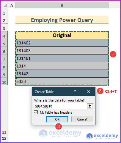
- So, it will transform the selected range into a table.
- Afterward, again select that cell range and from the Data tab, select From Table/Range.

- Therefore, the Power Query Editor window will appear.
- After that, we can see that the data type is changed automatically.
- Then, from the Close & Load option, select “Close & Load To…”.

- So, the Import Data dialog box will appear.
- Then, select cell B12 as the output under the Existing worksheet option.
- Finally, press OK.

- This will convert the green triangle to a number and the output will look like this.

Download Practice Workbook
Conclusion
We have shown you six easy methods to convert the green triangle to the number in Excel. If you face any problems regarding these methods, feel free to comment below. Moreover, you can also leave any feedback for us, so we can serve you better.
However, remember that our website implements comment moderation. Therefore, your comments may not be instantly visible. So, have a little bit of patience, and we will solve your query as soon as possible. Thanks for reading. Keep excelling!
Related Articles
- How to Convert Bulk Text to Number in Excel
- How to Convert Text to Number Using Formulas in Excel
- How to Fix Convert to Number Error in Excel
- How to Fix All Number Stored as Text in Excel
<< Go Back to Convert Text to Number in Excel | Learn Excel
Get FREE Advanced Excel Exercises with Solutions!
