How to Use the SUMIF Function between Two Values in Excel

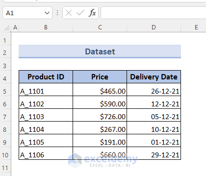
The dataset used for these methods contains three columns with the product ID, prices of the products, and delivery dates of a company’s products. 

SUMIF Function between Two Values in Excel: An Improvisation

Steps:

• Enter the following formula in Cell F5:

• Press Enter.

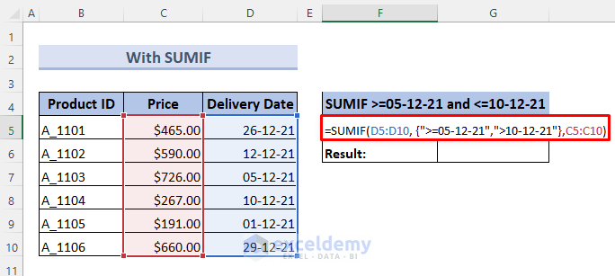
As the above formula works as an array formula, there are two outputs in two cells, F5 & G5.

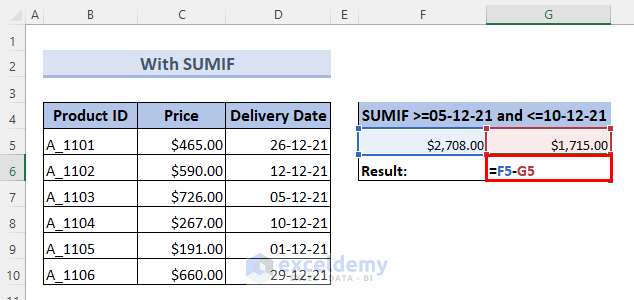
• Subtract the outputs. Type =F5-G5 in Cell G6.
  Or, you can generate the subtraction by entering (=) equal sign in Cell F6, drift and click the mouse on Cell F5, type (–) minus sign, then drift and click on Cell G5.
• Press Enter.

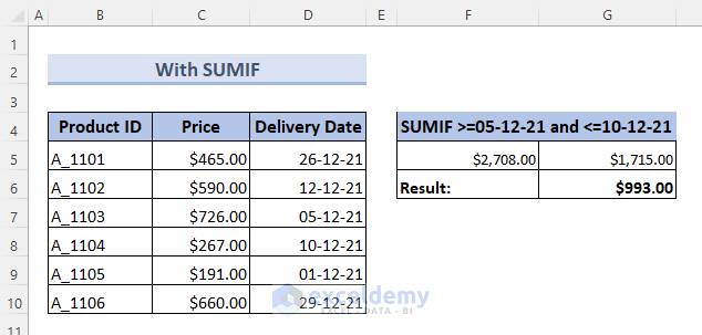
Finally, we have generated the results.

Method 1 – Using SUMIFS Between Two Values in Excel (Alternative to SUMIF Function)

1.1 With Numbers

Steps:

• Enter the following formula in Cell G5:

• Press Enter.

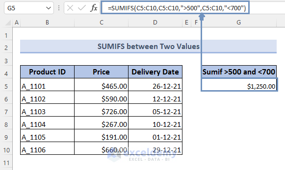
The formula looks for price values greater than 500 and less than 700. This brings out two values, 590 and 660. The result is $1250.

How Does the Formula Work?

The formula takes the criteria of two numbers, 500 and 700. To indicate greater or less, it used the signs “>” and “<” respectively before the numbers.
For the sum, the range is C5:C10, which contains the price of the products. Here, the sum and criteria range are the same.

1.2 With Cell References

Steps:

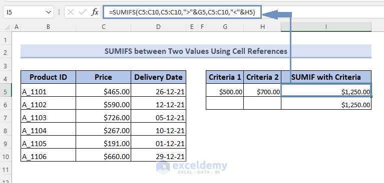
• Enter the numbers 500 and 700 in two different cells. We have written them in Cell G5 and Cell H5.
• Enter the formula of the SUMIFS function below in Cell I5:

• Press Enter.

Now, if you want to copy the result to a different worksheet, the result might get manipulated. To keep the formula and result intact:

• Enter the following formula:

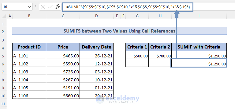
How the Formula Works

The formula takes the criteria of two cell references, G5 and H5, for the numbers 500 and 700. To indicate greater or less, it used the signs “>” and “<” respectively before the numbers. You can see “&” and sign after the operators to add the cell references along with the operators.
For the sum, the range is C5:C10, which contains the price of the products. Here, the sum and criteria range are the same.

1.3 With Named Range

Steps:

• Select the price data.

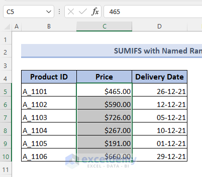
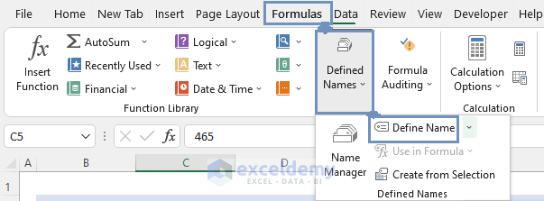
• From the Formulas tab, select Define Name, which you can find in the drop-down menu of Defined Names.

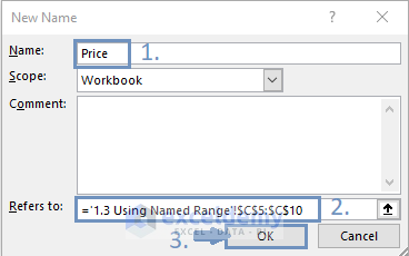
• A small box will come up. There you have to do the following things:
  • In the Name: section, write “Price”. You can write any name of your choice.
  • In the Scope: section, write Workbook ( by default)
  • Check the range and worksheet name in the Refers to section.
• Click OK.

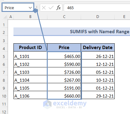
You will see the name Price by selecting the price data at the left corner of the worksheet. It is beside the formula bar.

• Enter the following formula in Cell F5:

• Press Enter to see the result.

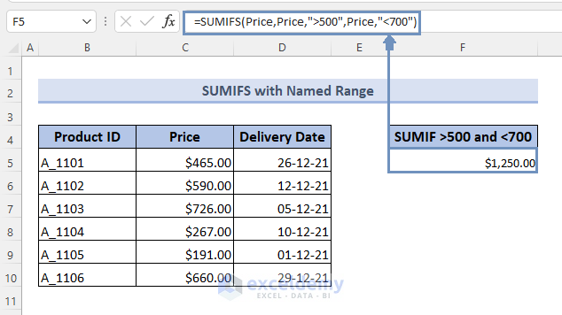
Here, you can select the range, and it will show the name Price instead of a cell reference. Again, you can simply write Price in the formula, and it will refer to the particular range C5:C10.

How the Formula Works

The formula takes the criteria of two numbers, 500 and 700. To indicate greater or less, it used the signs “>” and “<” respectively before the numbers.
For the sum, the range is C5:C10, which contains the price of the products. Here, the sum and criteria range are the same. Writing the price in the formula will directly select this range.

1.4 With Date Values

Steps:

• Enter the following formula in Cell F5:

• Press Enter to get the result.

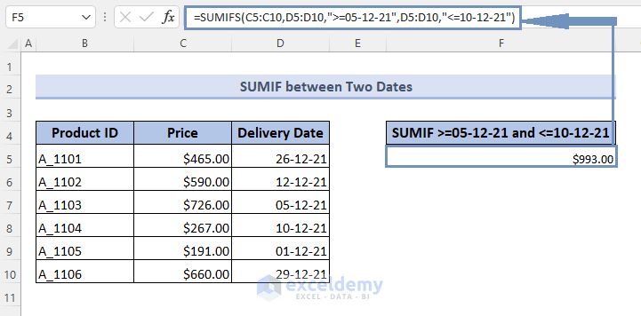
Here, we have set the criteria for the price having a delivery date on/after 05-12-21 and on /before 10-12-21.

How the Formula Works

The formula takes the criteria of two dates, 05-12-21 and 10-12-21. To indicate greater or less, including the dates, it used the signs “>=” and “<=” respectively before the numbers.
For the sum, the range is C5:C10, which contains the price of the products. The criteria range is D5:D10.

1.5 With Cell References

Steps:

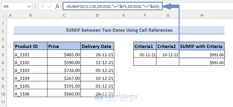
• Enter the dates 05-12-21 and 10-12-21 in Cell F5 and Cell G5.
• Enter the formula in Cell H5:

• Press Enter.

Use absolute cell references so that the formula and result remain the same while copying and pasting. For this, the formula becomes:

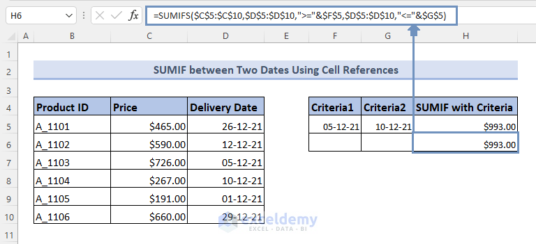
How the Formula Works

The formula takes the criteria of two cell references, F5 and G5, for the dates 05-12-21 and 10-12-21. To indicate greater or less, including the dates, it used the signs “>=” and “<=” respectively before the numbers. You can see “&” and sign after the operators to add the cell references along with the operators.
For the sum, the range is C5:C10, which contains the price of the products. The criteria range is D5:D10.

1.6 Using the TODAY Function

Steps:

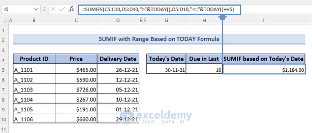
• Enter the formula =TODAY() in Cell G5.
• Enter 10 in cell H5.
• Enter the following formula in Cell I5:

• Press Enter.

For safety, you can use absolute references. In that case, the formula will be:

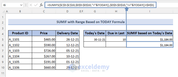
How the Formula Works

The formula with the TODAY function gives the present date.
The SUMIFS formula takes ranges for the sum as C5:C10 and criteria D5:D10.
It takes the TODAY() formula with operator “>” to indicate the dates after today. The operator concatenates with the formula by the “&” symbol.
The second TODAY() formula is added with 10 using the cell reference H5. This is concatenated with the operator “<=” with the “&” sign to indicate the dates less than or equal to 10 days, including today.

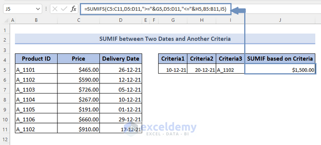
Method 2 – Applying Excel SUMIFS between Two Values with Multiple Criteria

Steps:

• Enter the dates 10-12-21 and 20-12-21 in Cell G5 and Cell H5.
• Enter the product ID A_1102 in Cell I5.
• Enter the following formula in Cell J5:

• Press Enter.

You can use absolute cell references in the formula for ease of copy and pasting.

The formula for this:

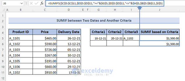
How the Formula Works

The formula takes the criteria of two dates, 05-12-21 and 10-12-21, using the cell references G5 and H5. To indicate greater or less, including the dates, it used the signs “>=” and “<=” respectively before the numbers. To concatenate the operators with the dates, the “&” sign is written before the cell references.
For the criteria of Product ID, the range is selected as A5:A10 and the criteria A_1102 is set using the cell reference I5.
For the sum, the range is C5:C10, which contains the price of the products. The criteria range is D5:D10.

Formula Not Working

If your formula isn’t working or showing an error, you might need the following checklist to find the problem.

1. Check the formats of dates and numbers.
2. Use correct operators with logic.
3. Follow the formula syntax accurately.
4. Make sure all the ranges are of the same size.

Things to Remember

You need to write the cell references and carefully insert the operators for particular criteria. If the criteria are not set with the dataset, it will return a zero (0) as a result.

Download the Practice Workbook

You can download the practice workbook from here.

<< Go Back to Excel SUMIF Function | Excel Functions | Learn Excel