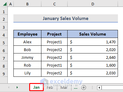
The sample Excel Workbook contains three Worksheets named Jan, Feb, and March. In each sheet, the B4:D9 cells contain the Employee, Project, and Sales Volume columns respectively.
The Jan worksheet contains the dataset for January Sales Volume.
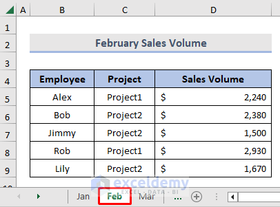
Feb sheet has the dataset for February Sales Volume.
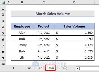
March sheet the dataset for March Sales Volume.
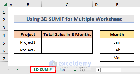
We will summarize the sales data in the worksheet shown below.
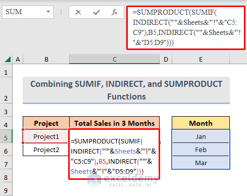
Method 1 – Combining SUMIF, INDIRECT, and SUMPRODUCT Functions
In order to use 3D Referencing with the SUMIF you will need to combine it with the INDIRECT and SUMPRODUCT functions to sum values from multiple worksheets.
Steps:
- Enter the following formula in cell C5.
=SUMPRODUCT(SUMIF(INDIRECT("'"&Sheets&"'!"&"C5:C9"),B5,INDIRECT("'"&Sheets&"'!"&"D5:D9")))Formula Breakdown:
- SUMIF(INDIRECT(“‘”&Sheets&”‘!”&”C5:C9”),B5,INDIRECT(“‘”&Sheets&”‘!”&”D5:D9”)) →Here C5:C9 is the required criteria range for each sheet to sum by, B5 is the specific criteria, D5:D9 is the same range of each sheet to sum. The Sheets function will return the sheet number and the INDIRECT function will help to return a valid reference.
- SUMPRODUCT(SUMIF(INDIRECT(“‘”&Sheets&”‘!”&”C5:C9”),B5,INDIRECT(“‘”&Sheets&”‘!”&”D5:D9”))) →This will multiply the values of the corresponding range and return the added value of each sheet.
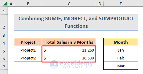
- Press ENTER and drag the “Fill Handle” down to fill.
- You will get the sum value according to the criteria from multiple worksheets.
Read More: How to Sum If Cell Contains Number and Text in Excel
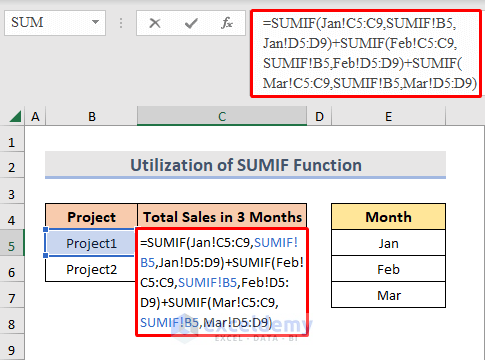
Method 2 – Utilizing SUMIF Function for 3D Referencing from Multiple Worksheets
Steps:
- Enter the following formula in cell C5.
=SUMIF(Jan!C5:C9,SUMIF!B5,Jan!D5:D9)+SUMIF(Feb!C5:C9,SUMIF!B5,Feb!D5:D9)+SUMIF(Mar!C5:C9,SUMIF!B5,Mar!D5:D9)Where,
- SUMIF(Jan!C5:C9,SUMIF!B5,Jan!D5:D9)→ In this part, the SUMIF function is summing value from range (Jan!C5:C9) with criteria from the cell (SUMIF!B5). Finally, summing the sum_range(Jan!D5:D9). Similarly, for Feb and Mar
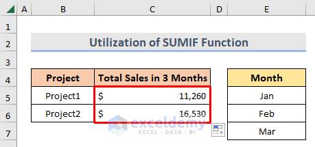
- Press ENTER and drag down the “Fill Handle”.
- You will get the final result.
How to Apply SUMPRODUCT Function Across Multiple Sheets
Steps:
- Enter the following formula in cell C5.
=SUM(SUMPRODUCT((Jan!C5:C9=SUMPRODUCT!B5)*(Jan!D5:D9)),SUMPRODUCT((Feb!C5:C9=SUMPRODUCT!B5)*(Feb!D5:D9)),SUMPRODUCT((Mar!C5:C9=SUMPRODUCT!B5)*(Mar!D5:D9)))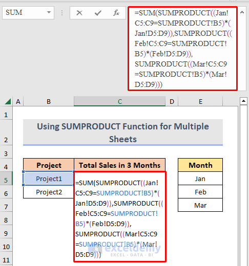
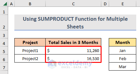
- Press the ENTER key and drag the “Fill Handle” down.
- You will get your desired result.
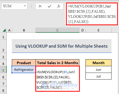
How to VLOOKUP and SUM Across Multiple Sheets
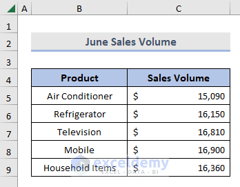
We have a dataset of the Sales Volume of multiple products for the month of June in a different worksheet.
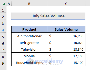
We also have the dataset for the month of July.
Steps:
- Enter the following formula in cell C5.
=SUM(VLOOKUP(B5,Jun!$B$5:$C$9,{2},FALSE),VLOOKUP(B5,Jul!$B$5:$C$9,{2},FALSE))Where,
- The VLOOKUP function will look up for values from a provided column ($B$5:$C$9) across multiple sheets.
- The SUM function will sum up the value extracted using the VLOOKUP function.
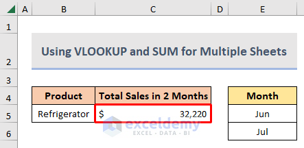
- Press ENTER and drag the “Fill Handle” down.
- You will get the total sales volume.
Download Practice Workbook
Related Articles
- How to Sum If Cell Contains Number in Excel
- How to Use Excel SUMIF with Greater Than Criterion
- How to Use Excel SUMIF to Sum Values Greater Than 0
- How to Use SUMIF to SUM Less Than 0 in Excel
- Sum If Greater Than and Less Than Cell Value in Excel
- How to Use Excel SUMIF Function Based on Cell Color
<< Go Back to Excel SUMIF Function | Excel Functions | Learn Excel
Get FREE Advanced Excel Exercises with Solutions!
