3D Referencing & External Reference in Excel

Creating 3D referencing in Excel within a formula involves referring to the same cell or the same range of cells, on different worksheets. Each of the sheets one uses to create the 3D referencing should have the same pattern and type of data.
Creating an external reference means that one is referring to a cell or a range of cells, in another Excel workbook or multiple workbooks.
Both 3D referencing & external reference in Excel are very efficient when one wants to collate data from multiple sheets or workbooks. So, let’s get started with simple examples, to illustrate how to create 3D referencing & external reference in Excel.

What Is 3D Referencing in Excel?

In Excel, users can utilize the 3D reference feature to select the very same cell from separate and numerous worksheets. By just choosing the title of the worksheet, we can choose the same cell or a particular range of cells from various sheets in Excel to serve as a reference.
For instance, we hold four worksheets called Jan, Feb, Mar, and Apr which each contain different integer values. Now, if we want to add the numbers from this worksheet without selecting a cell, we may use their names with the cell we want to add them to, like Jan: Apr. The range for the SUM function must be Jan: Apr!C3 if we wish to sum the value of cell location C3.
Here, you can get the list of functions compatible with 3D referencing in Excel.
The structure needed for a 3D reference within a formula is thus:
=Function(First_worksheet: Last_worksheet!cell_of_interest) in the case where it’s a single cell in the different worksheets, that is under evaluation.
Or
=Function(First_worksheet: Last_worksheet!range) in the case where it’s a range of cells in the different worksheets, that is under evaluation.

Introduction to Dataset

YouTube has more than 400 popular vlogging channels, devoted exclusively to beauty tutorials. While exploring the world of beauty vlogging on YouTube, one can find whole video tutorials on how to create a smokey eye effect, contour one’s cheeks, bridal makeup tips, cosplay makeup, and even stage makeup is covered. Many of these beauty vloggers have millions of subscribers and receive numerous sponsorship deals and endorsements.
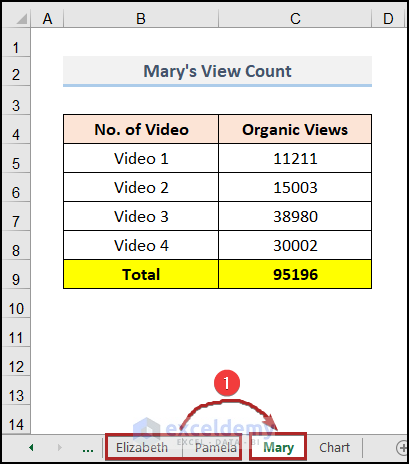
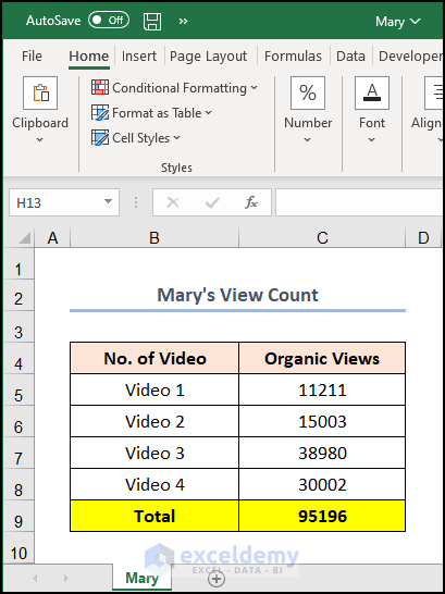
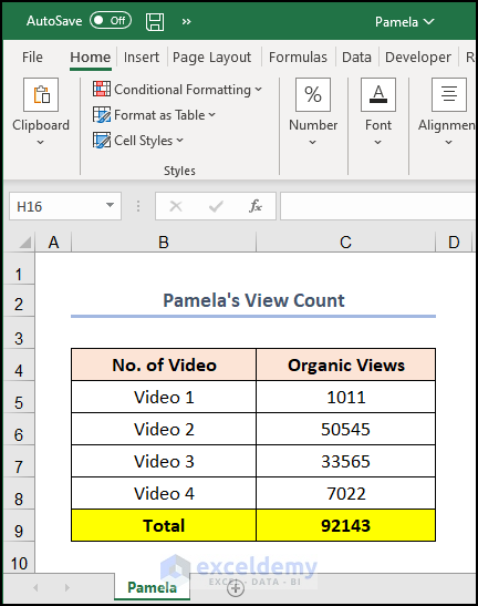
In our example, three hypothetical popular beauty vloggers Elizabeth, Mary, and Pamela, have received a sponsorship from a big hypothetical beauty brand. The sponsorship entails, each of the three bloggers creating four videos with the sponsor’s makeup products. The beauty brand is now measuring the exposure of its brand through the video views, obtained from the above three beauty vloggers. The source data is shown below.

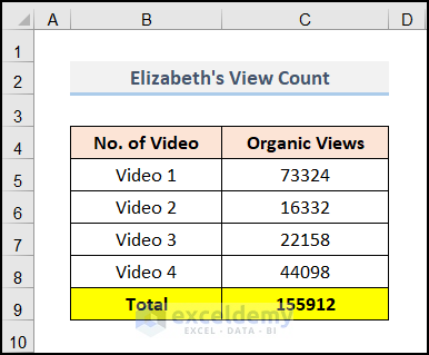
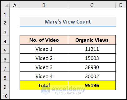
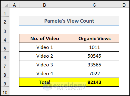
The workbook Utilizing 3D References contains five sheets, one named TotalBrandExposure, and the three other sheets contain the view counts and totals for each of the vlogger’s four videos, in cell C9. In the end, there is another sheet named Chart. All the sheets are in the same workbook.

Using 3D Referencing in Excel: 3 Examples

On the TotalBrandExposure sheet, we’d like to create 3D referencing in Excel that totals the combined amount of views as well as finds the minimum view for the three vloggers. So, let’s go through the examples one by one.
Here, we have used Microsoft Excel 365 version, you may use any other version according to your convenience.

Example 01: 3D Referencing with SUM Function

In our first example, we would like to know the total views generated by the three vloggers. We will thus create a SUM formula and use a 3D reference, in order to do this. To do this, you may follow the below steps.

📌 Steps:

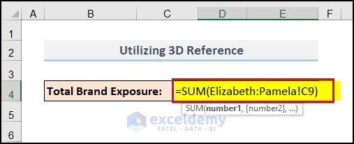
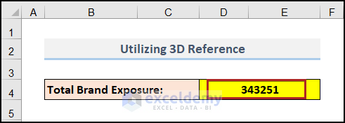
• At the very beginning, select cell D4 in the TotalBrandExposure sheet.
• Following this, write down the following formula.

We start by referring to the first sheet in the formula, we then add a colon.  The last sheet we want to refer to follows the colon. All sheets in between the first sheet and the last sheet will also be included in the calculation. An exclamation mark is then added, followed by the cell of interest, which in this case is cell C9.
The formula will total each of the amounts in C9 for the first sheet specified, the last sheet specified, and all the sheets in between, so in other words Elizabeth’s, Mary’s and Pamela’s total views will be added.

• After that, we obtain a value of 343251 views upon pressing ENTER, which is the sum of the total views of the three vloggers.

Read More: How to Use SUM and 3D Reference in Excel

Example 02: 3D Referencing with MIN Function

3D referencing is supported by the SUM, AVERAGE, AVERAGEA, COUNT, COUNTA, MAX, MAXA, MIN, MINA, PRODUCT, STDEV, STDEVA, STDEVP, STDEVPA, VAR, VARA, VARP, and VARPA functions only.

We are now going to use the MIN function in conjunction with a 3D reference, in order to see what the minimum value in the range C5:C8, for the three different vloggers, is. In other words, out of the videos made by the three vloggers, which vlogger has the lowest view count.

📌 Steps:

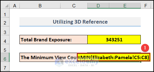
• At first, on the TotalBrandExposure sheet, select cell D6.
• Later, paste the following formula into that cell.

This time we are using a 3D reference with a range, and the MIN function, evaluates the C5:C8 range in the sheets specified in the reference.

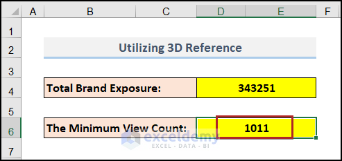
• At this time, you can get a value of 1011 upon pressing ENTER, which is the minimum value across the C5:C8 range in the three sheets.

Example 03: Inserting Chart in Excel

In the above two examples, we’ve seen the use of 3D reference in performing calculations. But the field of performance of this isn’t bound to that. Using 3D reference, we can insert a chart in Excel. It’s simple & easy, just follow along.

📌 Steps:

• Firstly, add a new blank worksheet Chart in the workbook.

• Secondly, go to the Insert tab.
• Then, click on the Insert Column or Bar Chart drop-down icon on the Charts group.
• After that, select 2-D Clustered Column from the available options.

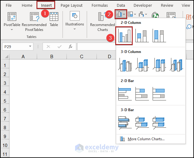
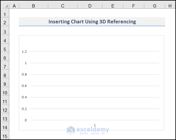
Thus, it inserts a blank chart in the worksheet.

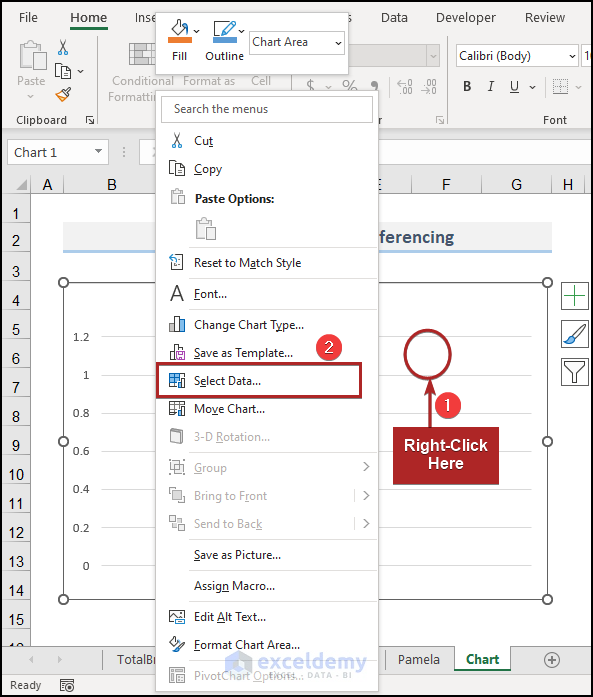
• Thirdly, right-click anywhere on the chart area.
• Then, from the context menu, choose the option Select Data.

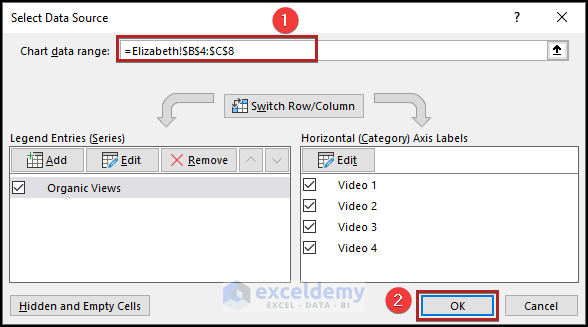
Hence, the Select Data Source dialog box opens.

• Here, in the Chart data range box, give the reference of cells in the B4:C8 range in the Elizabeth worksheet.
• Correspondingly, click OK.

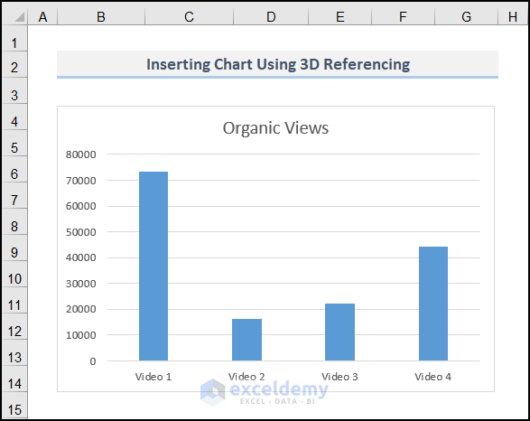
• In this way, we get a clean and precise chart of Elizabeth’s Organic Views for each video.

When Does 3D Referencing Change?

In this section, we’ll talk about the changes in 3D references. Here, you‘ll get the answer to when 3D referencing changes. Also, you’ll get to know the consequences of these changes on results.

1. If You Insert New Worksheet

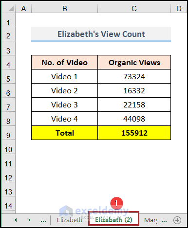
Let’s say you have created a copy of the worksheet Elizabeth between the worksheets Elizabeth and Mary. Excel will name it Elizabeth (2) automatically as there is another sheet available with the same name in the corresponding workbook.

Now, move to the worksheet TotalBrandExposure and you’ll find a new value of Total Brand Exposure.

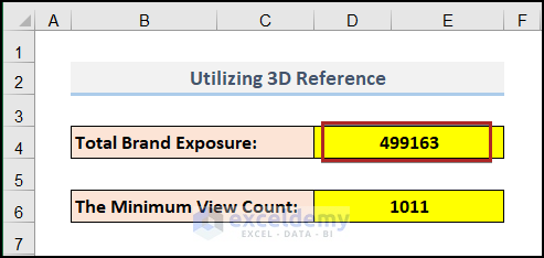
It happens because we put a new worksheet between the first and last sheet of the reference. So, Excel is getting it into the calculation. As a result, the Total Organic Views of Elizabeth is getting summed up twice and created the final value of 499163 instead of 343251.

2. If You Move Worksheet

Let’s assume, you moved the worksheet Mary from the middle of Elizabeth and Pamela to the right of Pamela.

So, what do you think? What will happen? The Total Brand Exposure gets decreased.

Why did it happen? Because we altered the position of sheet Mary from between the first sheet and the last sheet of the reference. Therefore, Excel excludes it from the calculation. Consequently, it’s displaying the value as 248055 instead of 343251.

How to Create a 3D Reference in Excel with Names

To ease the use of 3D reference, we also can define names in Excel. To do so, go through the following simple steps.

📌 Steps:

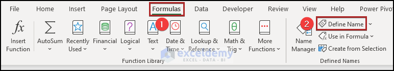
• First of all, jump to the Formulas tab.
• Secondly, select Define Name on the Defined Names group.

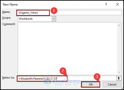
Immediately, the New Name dialog box pops up.

• Here, write the Name as Organic_Views.
• Then, put =Elizabeth:Pamela!$C$5:$C$8 in the box of Refers to.
• Lastly, click OK.

• At this moment, go to the worksheet TotalBrandExposure.
• After that, select cell D6 and paste the following formula.

• Then, press ENTER.

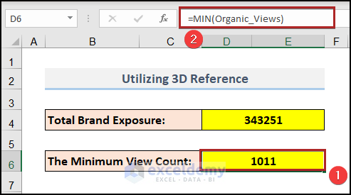
Here, we’re getting the same result as Example 02 using a predefined name.

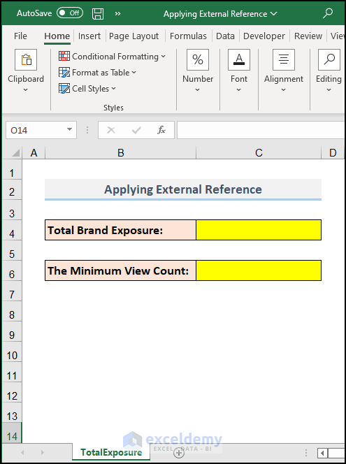
2 Examples of Applying External Reference in Excel

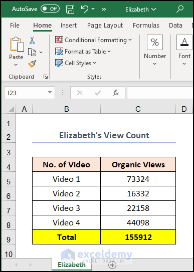
We now will consider the situation, where we have one master workbook called Applying External Reference and three other different workbooks, containing the view count data from the three individual vloggers. So, basically, we have one master workbook called Applying External Reference, one workbook named Elizabeth, the other named Mary, and the last one named Pamela. The source data is shown below.

Now, we’ll perform some calculations using external references using these workbooks. So, let’s explore them one by one.

Example 01: Calculating Sum from Different Workbooks

We are now going to use the SUM function in conjunction with an external reference, in order to see what the total view count for all three vloggers, is. So, let’s see it in action.

📌 Steps:

• Initially, open all four workbooks and keep them in different tabs.
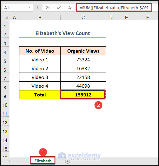
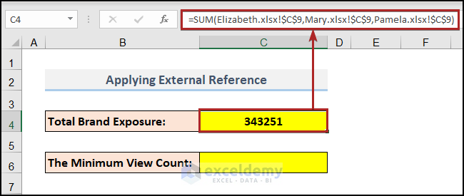
• In the worksheet called TotalExposure, in cell C4, start the formula with =SUM.
• Then, open parenthesis and then navigate to the workbook called Elizabeth and select cell C9, as shown below.

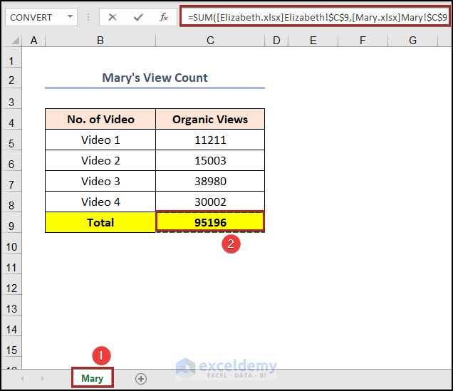
• After that, insert a comma in the formula bar, and then navigate to the workbook called Mary and select cell C9, as the screenshot shows below.

• Again, type a comma in the formula bar and then navigate to the workbook called Pamela and select cell C9 as the following image.

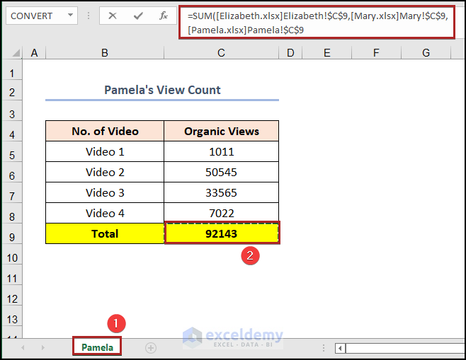
• While still in the Pamela workbook, close the parenthesis in the formula bar and press ENTER as shown below.

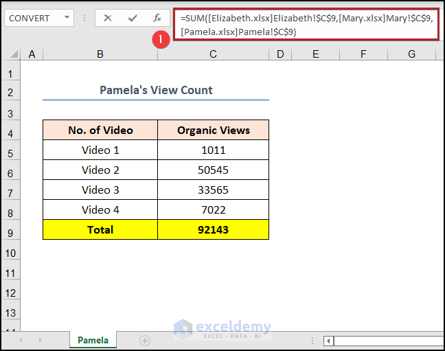
• Upon pressing ENTER, one is returned back to cell C4, in the TotalExposure worksheet and the combined view count is delivered, save your workbook once completed.

Example 02: Finding the Minimum Value from Different Workbooks

We are now going to use the MIN function in conjunction with an external reference, in order to see what the minimum value in the range C5:C8 for the three different vlogger’s data is. So, without further delay, let’s see how we do it.

📌 Steps:

• Primarily, open all four workbooks.
• Secondarily, in the worksheet called TotalExposure, in cell C6, start the formula with =MIN.
• Then, open parenthesis and navigate to the workbook called Elizabeth and select the range C5:C8, as shown below.

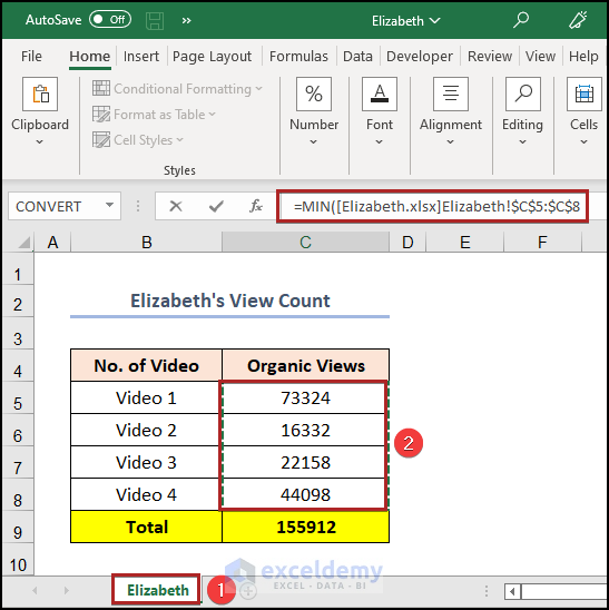
• After that, type a comma in the formula bar, and then navigate to the workbook called Mary and select the range C5:C8, as in the following screenshot.

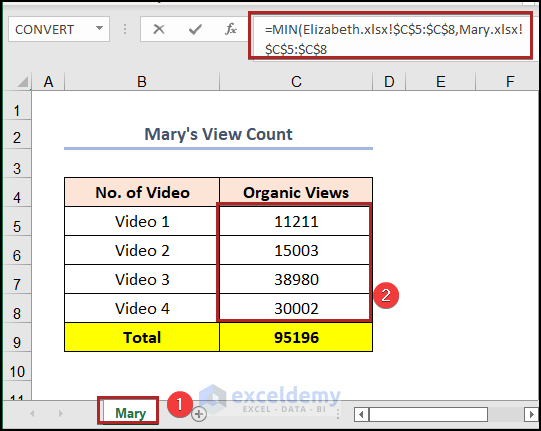
• Also, insert a comma in the formula bar, and then navigate to the workbook called Pamela and select the range C5:C8 as in the image shown below.

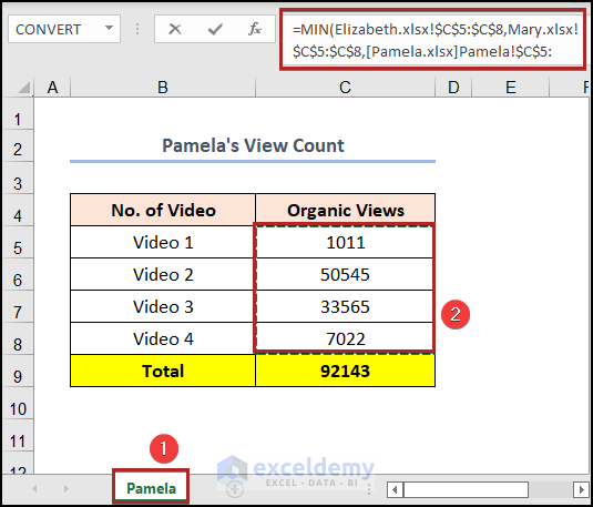
• While still in the Pamela workbook, close the parenthesis and press the ENTER key as shown below.

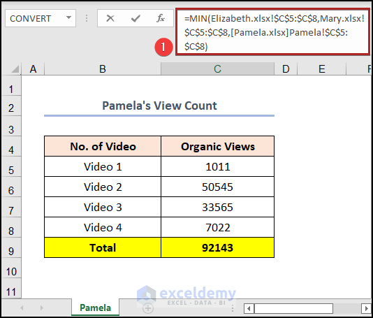
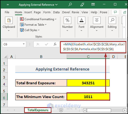
• Upon pressing ENTER, one is returned back to cell C6 in the TotalExposure worksheet and the minimum result is delivered. Then save your workbook once completed.

Updating Links of External Reference

When opening workbooks, that contain links to other workbooks, one will be asked whether one wants to update the master workbook, in order to reflect any changes made in the linked data, or not to update as shown below.

Usually one would want to update the master workbook with the latest data.
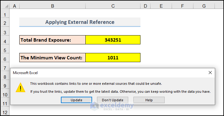
Note: When the source workbooks are not opened the formula bar will show the external reference with the entire path to the workbooks.
To update the workbook always, follow the steps below carefully.

📌 Steps:

• First, proceed to the Data tab.
• Secondly, click on Edit Links on the Queries & Connections group.

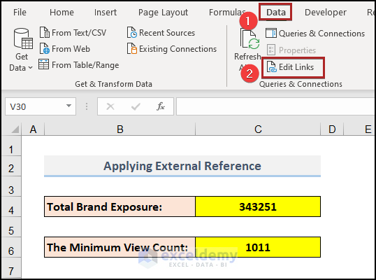
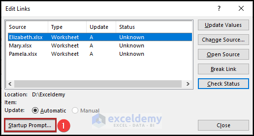
Instantly, the Edit Links wizard appears.

• Here, select Startup Prompt on the left-below side of the box.

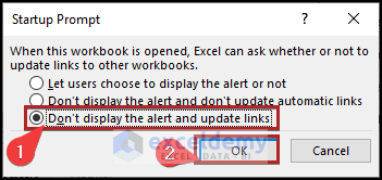
Correspondingly, the Startup Prompt dialog box pops up.

• Then, select Don’t display the alert and update links.
• Lastly, click OK.

Again, it returns to the Edit Links wizard.

• Finally, click on Close.

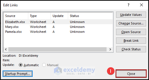
• Then, save the workbook.

The next time, you open the workbook Applying External Reference, the alert will not be shown, however, the values will be updated with any changes made in the source workbooks Elizabeth, Mary, and Pamela.

Read More: 3D Reference Not Working in Excel

Bonus: Free Template

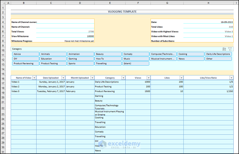
We have also included a FREE Vlogging Excel Template, which will allow you to record vlogging data from your YouTube channel or other vlogging social media channels.

Template Description:

• You can input your name, the name of the channel, your total number of subscribers, and the desired view count milestone, as well as the individual video data in the Table provided.
• This template calculated the current date automatically, as is the video with the highest number of views, and the video with the highest number of likes.  We can also get the Total views and Total likes calculated automatically. You will also get whether or not you have met your desired Viewing Milestone, based on the data in the Table.
• It will deliver the name of the video with the most Likes automatically as is the name of the video with the most Views. This is especially handy in cases where one has many rows of Table data.
• You can enter individual video data in the table and input the Name of the Video and the Date when you uploaded it. Once you input the Date, you can get the Month automatically in the next column.
• You can choose a category from the Category options, and enter the view count for the video at hand, and the number of likes. Then, you’ll find the like-to-view ratio automatically.
• You can also filter the Table using the slicer which filters data on the Category Column.

Download Practice Workbooks

You may download the following Excel workbooks for a better understanding and to practice yourself.

Conclusion

This article provides easy and brief descriptions of 3D referencing & external reference in Excel. . Use the Template if you need it. Thank you for reading this article, we hope this was helpful. Please let us know in the comment section if you have any queries or suggestions.

<< Go Back to 3D Reference | Cell Reference in Excel | Excel Formulas | Learn Excel