Top 100 MCQ of Excel: Test Your Skills

In this article, you will find the top 100 MCQ of Excel to test your skills. Most of the questions are very basic. As a result, anyone with a basic understanding of Excel will be able to answer the questions. These questions will be helpful for job and academic examinations. Moreover, you should know the following: introduction to Excel VBA, enable the Developer tab, the basics of an Excel spreadsheet, use of the INDEX-MATCH formula, use of the Excel Chart options, custom format cells, application of Data Validation, application of the AGGREGATE, AVERAGE, AVERAGEIF, CEILING.MATH, COUNT, COUNTBLANK, IF, IFS, COUNTIF, COUNTA, COUNTIFS, DATEDIF, DAY, FIND, IFERROR, LEN, MROUND, RAND, RANDBETWEEN, ROW, ROWS, SUM, SUMIF, TODAY, VLOOKUP, and XLOOKUP functions to solve them. You should use at least Excel 2019 to solve the problems without any issues.

Download Practice Workbook

Problem Overview

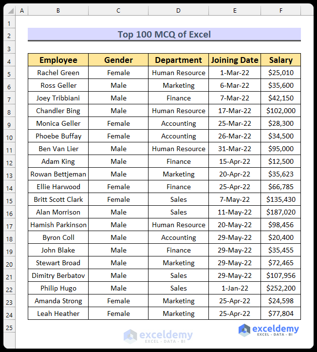
The Excel file contains the top 100 MCQs of Excel and their corresponding answers. The questions are provided in the “Problem” sheet. Additionally, the answers are highlighted in the “Solution” sheet. We can see a snapshot of the sample dataset for this article below. This dataset represents the data for twenty employees of a particular company. You can practice the correct answers to the MCQ on the dataset. You can provide your answer (by typing or selecting from the dropdown list) in the “I” column. If it is correct, you will get a green checkmark in the “J” column.

Now, let’s go through the top 100 MCQs of Excel. You can provide your answers either by typing or using the dropdown list in the Excel file containing the top 100 MCQs in Excel.

• Q1. What is the maximum number of worksheets in Excel?
  • (a) 256
  • (b) 65
  • (c) There is no limitation
  • (d) 128
• Q2. How do you select an entire row in Excel?
  • (a) Click on the row number
  • (b) Press Ctrl+Alt+3
  • (c) Press Alt+Space Bar
  • (d) Press Shift+Dot
• Q3. To bring up the custom cell Formatting press –
  • (a) Ctrl+1
  • (b) Ctrl+2
  • (c) Ctrl+3
  • (d) Ctrl+4
• Q4. To find the maximum salary, you can use –
  • (a) =MAX(F5:F24)
  • (b) =LARGE(F5:F24,1)
  • (c) =AGGREGATE(4,0,F5:F24)
  • (d) All of the above
• Q5. You can find the mean of the salaries using –
  • (a) =AGGREGATE(2,0,F5:F24)
  • (b) =AVERAGE(F5:F24)
  • (c) =MEAN(F5:F24)
  • (d) All of the above
• Q6. Which formula will return 0 –
  • (a) =COUNTA(C5:C24)
  • (b) =COUNT(C5:C24)
  • (c) =COUNTBLANK(C5:C24)
  • (d) None of these
• Q7. How many functions are included in the AGGREGATE function –
  • (a) 17
  • (b) 18
  • (c) 19
  • (d) 20
• Q8. To find the string size (number of characters) for the name column, you will use –
  • (a) =LEN(B5:B24)
  • (b) =SIZE(B5:B24)
  • (c) =STRINGLENGTH(B5:B24)
  • (d) =LENGTH(B5:B24)
• Q9. If you want to count the number of employees whose name begins with R, you can use –
  • (a) =COUNTIF(B5:B24,R*)
  • (b) =COUNTIF(B5:B24,”R*”)
  • (c) =COUNTIF(B5:B24,”R”)
  • (d) =COUNTIF(B5:B24,”*R”)
• Q10. To calculate the space position in the name column, you can use –
  • (a) =FIND(” “,B5:B24,1)
  • (b) =SEARCH(” “,B5:B24,1)
  • (c) =AGGREGATE(” “,B5:B25,1)
  • (d) Both a&b
• Q11. The difference between the SEARCH and FIND function is –
  • (a) The FIND function is case-sensitive and the SEARCH function is not
  • (b) The SEARCH function is case-sensitive and the FIND function is not
  • (c) There is no difference between them, only for compatibility, both are listed
  • (d) None of these
• Q12. Which Function can be used to Find the Number of Females?
  • (a) COUNTIFS
  • (b) COUNTIF
  • (c) COUNT
  • (d) Both a & b
• Q13. The function to find the highest salary value is –
  • (a) MAX
  • (b) MAXIMUM
  • (c) AGGREGATE
  • (d) Both a & c
• Q14. The total value of salary for the male employees can be calculated by using –
  • (a) SUMIF
  • (b) IFS
  • (c) MAX
  • (d) INDEX-MATCH
• Q15. To find the employee who received the most salary, you will use the following formula –
  • (a) =INDEX(B5:B24,MATCH(MAX(F5:F24),F5:F24,0))
  • (b) =INDEX(B5:B24,MATCH(MAX(F5:F24),F5:F24,1))
  • (c) =INDEX(B5:B24,MAX(F5:F24),0)
  • (d) =INDEX(B5:B24,MATCH(MAX(F5:F24),F5:F24,-1))
• Q16. To find the distinct job department names, you can use –
  • (a) AGGREGATE
  • (b) UNIQUE
  • (c) Combination of IFERROR, INDEX, MATCH
  • (d) Both b & c
• Q17. To extract the day value from the Date Joined column, which of the following features can be used?
  • (a) DAY Function
  • (b) Insert an adjacent helper column and use Flash Fill
  • (c) LEFT Function
  • (d) Both a,b & c
• Q18. Which function can be used to determine the number of empty cells in the dataset?
  • (a) COUNT
  • (b) COUNTA
  • (c) COUNTBLANT
  • (d) COUNTBLANK
• Q19. Using which function from the list you can return a random name –
  • (a) =INDEX(B5:B24,MATCH(RANDBETWEEN(1,20),B5:B24,0))
  • (b) =INDEX(B5:B24,RANDBETWEEN(1,20))
  • (c) =INDEX(B6:B25,RAND())
  • (d) =INDEX(B6:B25,RAND(20))
• Q20. To determine the number of salary greater than $100,000 AND dates joined after 30th April, the following formula needs to be used –
  • (a) =COUNTIFS(F5:F24,”>100000″,E5:E24,”>44681″)
  • (b) =COUNTIF(F5:F24,”>100000″)+COUNTIF(E5:E24,”>44681″)
  • (c) Both a & b
  • (d) None of these
• Q21. To determine the number of salary greater than $100,000 OR dates joined after 30th April, the following formula needs to be used –
  • (a) =COUNTIFS(F5:F24,”>100000″,E5:E24,”>44681″)
  • (b) =COUNTIF(F5:F24,”>100000″)+COUNTIF(E5:E24,”>44681″)
  • (c) Both a & b
  • (d) None of these
• Q22. To calculate the average salary by the male employees, the following formula need to be used –
  • (a) =AVERAGEIF(C5:C24,”Male”,F5:F24)
  • (b) =AVERAGEIFS(C5:C24,”Male”,F5:F24)
  • (c) =IF(C5:C24=”Male”,AVERAGE(F5:F24),””)
  • (d) =MEANIF(C5:C24,”Male”,F5:F24)
• Q23. To find the arithmetic mean, you can use the following function –
  • (a) MEAN
  • (b) AVERAGE
  • (c) GEOMEAN
  • (d) MIDPOINT
• Q24. Shortcut to apply the SUM function is –
  • (a) Alt+=
  • (b) Ctrl+=
  • (c) Shift+=
  • (d) Ctrl+Alt+=
• Q25. To return value from the left side of the matched value, we can use –
  • (a) VLOOKUP Function
  • (b) Combination of VLOOKUP and IF Functions
  • (c) HLOOKUP Function
  • (d) ZLOOKUP Function
• Q26. Which formula is correct for returning the name of the employee for the $25,010 salary?
  • (a) =VLOOKUP(F5,IF({1,0},F5:F24,B5:B24),2,0)
  • (b) =ZLOOKUP(F5,F5:F24,B5:B24)
  • (c) =XLOOKUP(F6,F5:F24,B5:B24)
  • (d) Both a&c
• Q27. The cell C15 is empty and F15 is $135,430. So, the output of =C15*F15 is –
  • (a) $135,430
  • (b) 0
  • (c) #VALUE!
  • (d) #DIV/0
• Q28. Which of the following functions will you use to determine the number of values in the Salary column?
  • (a) NUM
  • (b) NUMBER
  • (c) COUNT
  • (d) None of these
• Q29. If you want show the current date with time, you can use –
  • (a) =NOW()
  • (b) =TODAY()
  • (c) Both
  • (d) None of these
• Q30. Which of the formulas will you use to round up the salary figure from cell F17 to the nearest thousand?
  • (a) =MROUND(F17,1000)
  • (b) =FLOOR.MATH(F17,1000)
  • (c) =CEILING.MATH(F17,1000)
  • (d) =ROUNDUP(F17,1000)
• Q31. You can assign sequential serial number (1,2,3, etc.) to the rows by using the formula and AutoFill –
  • (a) =ROWS($B$5:B5)
  • (b) =ROWS(B5)
  • (c) =ROW(B5)-3
  • (d) Both a&c
• Q32. Which of the following are not valid Excel functions –
  • (a) NUM
  • (b) MEANS
  • (c) TRUE
  • (d) Both a&b
• Q33. Which of the following functions is available but not shown in Excel Tooltip?
  • (a) DATEVALUE
  • (b) DATEDIF
  • (c) KLOOKUP
  • (d) DCOUNT
• Q34. If you want to fix a cell reference, you will use –
  • (a) $
  • (b) !
  • (c) *
  • (d) %
• Q35. The Not Equal operator in Excel is –
  • (a) =!
  • (b) <>
  • (c) !=
  • (d) ||
• Q36. Circular reference in Excel formula is –
  • (a) A reference that relies on itself
  • (b) A type of the absolute cell reference
  • (c) A reference that Speeds up calculation
  • (d) None of these
• Q37. To fill down a formula, you need to use the following shortcut –
  • (a) Ctrl+D
  • (b) Alt+D
  • (c) Shift+D
  • (d) Ctrl+Alt+D
• Q38. Which of the following shortcuts can be used to use the Flash Fill feature?
  • (a) Ctrl+F
  • (b) Ctrl+E
  • (c) Alt+E
  • (d) Alt+F
• Q39. If you want to display the remainder after you divide 100 by 3, then you should use –
  • (a) =MOD(100,3)
  • (b) =DIV(3,100)
  • (c) =MODE(100,3)
  • (d) =REMAINDER(100,3)
• Q40. To concatenate values in the formula, you need to use –
  • (a) Semicolon (;)
  • (b) Comma (,)
  • (c) Ampersand (&)
  • (d) Pipe (|)
• Q41. Which is the latest lookup function?
  • (a) KLOOKUP
  • (b) XLOOKUP
  • (c) VLOOKUP
  • (d) LOOKUP
• Q42. A formula must begin with –
  • (a) =
  • (b) +
  • (c) –
  • (d) (
• Q43. Which of the following formula contains an error?
  • (a) =F7+F8
  • (b) =F9+F11
  • (c) (F9+F11)
  • (d) No error
• Q44. To find the output of the formula, you need to select the full formula or a portion of it and need to press X to show the output. Here X is – 
  • (a) F7
  • (b) F8
  • (c) F9
  • (d) F10
• Q45. To refer to a cell reference from another worksheet, you can –
  • (a) navigate to the sheet and click on that cell
  • (b) type the sheet name, add !, and include the cell address
  • (c) both of these
  • (d) It is not possible in Excel
• Q46. Which of the following functions was introduced in Excel 2019?
  • (a) UNIQUE
  • (b) IFS
  • (c) FLOOR.MATH
  • (d) XLOOKUP
• Q47. Which of the following functions can handle all kinds of errors?
  • (a) IFNA
  • (b) IFERROR
  • (c) ISERROR
  • (d) ALLERROR
• Q48. In the VBA Cells function, the argument is Cells (x, y), which means –
  • (a) x = row number, y = column number
  • (b) x = column number, y = row number
  • (c) x = row index, y = column index
  • (d) x = column index, y = row index
• Q49. To remove extra spaces, you can use the function –
  • (a) TRIM
  • (b) TRUNC
  • (c) CODE
  • (d) DELETE
• Q50. If there is a VBA code in your Excel file, then you should save the file as ____ format –
  • (a) .xlsx
  • (b) .xls
  • (c) .xlsm
  • (d) .csv
• Q51. To insert chart from a data selection, you will need to press – 
  • (a) F5
  • (b) F7
  • (c) F11
  • (d) F2
• Q52. If there is a Green triangle in the top left corner of the cell, then it signifies –
  • (a) There is a note in that cell
  • (b) The cell is formatted as a number
  • (c) There is no error on that cell
  • (d) There is a circular reference
• Q53. If there is a Red triangle in the top right corner of the cell, then it signifies –
  • (a) There is a note in that cell
  • (b) The cell is formatted as text
  • (c) There is an error on that cell
  • (d) There is a circular reference
• Q54. The maximum height of a row is 
  • (a) 409.5 Units
  • (b) 403.5 Units
  • (c) 410 Units
  • (d) 412 Units
• Q55. For showing distribution of data, you should use –
  • (a) Pie Chart
  • (b) Line chart
  • (c) Bar Chart
  • (d) Histogram
• Q56. To open the Spelling dialog box, you need to press – 
  • (a) F5
  • (b) F7
  • (c) F11
  • (d) F2
• Q57. The first cell of the Excel Workbook is –
  • (a) AA
  • (b) A1
  • (c) a1
  • (d) A
• Q58. The executable file to open Windows version of MS Excel is –
  • (a) EXCEL.exe
  • (b) MSEXCEL.exe
  • (c) WINEXCEL.exe
  • (d) EXCEL<version number>.exe
• Q59. To repeat the previous action, you will need to press on –
  • (a) F4
  • (b) F5
  • (c) F6
  • (d) F8
• Q60. The first version of Excel released on Microsoft Windows is –
  • (a) Excel 1.0
  • (b) Excel 2.0
  • (c) Excel 3.0
  • (d) Excel Alpha
• Q61. SUMX2MY2 is an Excel function. Here, M after X2 means –
  • (a) Minus
  • (b) Multiple
  • (c) Mode
  • (d) Modulus
• Q62. To find the highest common factor in Excel, you need to use –
  • (a) HCF Function
  • (b) LCM Function
  • (c) GCD Function
  • (d) None of these
• Q63. Which of the following is a shortcut for moving to the previous procedure in the VBE?
  • (a) Ctrl+Alt+Up Arrow
  • (b) Ctrl+Shift+Up Arrow
  • (c) Shift+Up Arrow
  • (d) Ctrl+Up Arrow
• Q64. Which is NOT a function category?
  • (a) Cube
  • (b) Information
  • (c) Web
  • (d) Mechanical Engineering
• Q65. The default row height of Excel is –
  • (a) 15
  • (b) 20
  • (c) 25
  • (d) 30
• Q66. Which of the following is a shortcut for running the current VBA code in Excel?
  • (a) F4
  • (b) F5
  • (c) F6
  • (d) F3
• Q67.  Which of the following functions is a Valid function?
  • (a) SUMX2PY2
  • (b) SUMX2MY2
  • (c) SUMXMY
  • (d) both a&b
• Q68. How do you undo an action in Excel?
  • (a) Ctrl+Z
  • (b) Ctrl+Y
  • (c) Ctrl+P
  • (d) Ctrl+K
• Q69. The default column width is –
  • (a) 8.41 unit
  • (b) 8.42 unit
  • (c) 8.43 unit
  • (d) 8.44 unit
• Q70. If you press Ctrl+0 it will –
  • (a) Hide the selected row
  • (b) Hide the selected column
  • (c) Open Cell Format dialog box
  • (d) Activate Format Painter feature
• Q71. The following shortcut key will open the Find and Replace dialog box, and activate the Replace tab –
  • (a) Ctrl+H
  • (b) Ctrl+R
  • (c) Ctrl+F
  • (d) Alt+F
• Q72. By default, the number of sheet in the workbook of Excel 365 is –
  • (a) 1
  • (b) 2
  • (c) 3
  • (d) 4
• Q73. How do you access the VBA editor in Excel?
  • (a) Press F11
  • (b) Go to the Insert tab and click on the VBA button
  • (c) Go to the Developer tab and click on the Visual Basic button
  • (d) All of the above
• Q74. How do you insert a note in Excel?
  • (a) Ctrl+Alt+M
  • (b) Shift+F2
  • (c) Ctrl+Alt+N
  • (d) Shift+F3
• Q75. Which of the following is NOT a type of data validation rule?
  • (a) Whole number
  • (b) Date
  • (c) Custom
  • (d) None of the above
• Q76. How do you select an entire column in Excel?
  • (a) Ctrl+Space Bar
  • (b) Shift+Space Bar
  • (c) Ctrl+Shift+Down Arrow
  • (d) Ctrl+Shift+UP Arrow
• Q77. For showing composition of something, you should use –
  • (a) Pie Chart
  • (b) Line chart
  • (c) Scatter Chart
  • (d) Histogram
• Q78. What is the function of the IFERROR function in Excel?
  • (a) It returns a value if a cell contains an error
  • (b) It hides errors in a cell
  • (c) It replaces errors in a cell with a specified value
  • (d) It displays a custom error message in a cell
• Q79. How do you redo an action in Excel?
  • (a) Ctrl+Z
  • (b) Ctrl+P
  • (c) Ctrl+S
  • (d) Ctrl+Y
• Q80. In which of the following cases would the formula =SUM(F5:F24) return an error?
  • (a) F5:F24 contains text values
  • (b) F5:F24 contains a mix of text and numeric values
  • (c) F5:F24 contains only numeric values
  • (d) F5:F24 is an empty range
• Q81. To insert the current date without time, you can –
  • (a) Press Ctrl+;
  • (b) Use TODAY Function
  • (c) Use NOW Function
  • (d) both a&b
• Q82. For comparison of data, you should use –
  • (a) Pie Chart
  • (b) Line chart
  • (c) Treemap
  • (d) Histogram
• Q83. How do you paste a cell in Excel?
  • (a) Ctrl+V
  • (b) Ctrl+P
  • (c) Ctrl+K
  • (d) Ctrl+X
• Q84. To switch to the next Sheet you can press –
  • (a) Ctrl+Page Down
  • (b) Shift+Page Down
  • (c) Alt+Page Down
  • (d) Shift+Alt+Right Arrow
• Q85. How do you go to the first cell (A1) in Excel?
  • (a) Alt+Home
  • (b) Ctrl+Page Up
  • (c) Ctrl+Home
  • (d) Ctrl+Shift+Home
• Q86. Which of the following is NOT a valid Excel function?
  • (a) MINUS
  • (b) ADD
  • (c) SUBTRACT
  • (d) All of the above
• Q87. Which of the following is NOT a valid Windows Excel version?
  • (a) Excel 2011
  • (b) Excel 97
  • (c) Excel 95
  • (d) Excel 2021
• Q88. How do you select the entire worksheet in Excel?
  • (a) Ctrl+D
  • (b) Ctrl+A
  • (c) Ctrl+K
  • (d) Ctrl+Alt+A
• Q89. If you select a range of cells and type something, then pressing a specific shortcut will copy the value to the selected range. Now, that shortcut key is –
  • (a) Shift+Enter
  • (b) Ctrl+Enter
  • (c) Alt+Enter
  • (d) None of these
• Q90. When you move your cursor to the bottom right corner of a cell, it turns into a plus (+) sign. This icon is known as –
  • (a) AutoFill Tool
  • (b) Fill Handle
  • (c) Fill Tool
  • (d) Drag Handle
• Q91. Which of the following is an absolute cell reference?
  • (a) F15
  • (b) F$15
  • (c) $F$15
  • (d) $F15
• Q92. How do you copy a cell in Excel?
  • (a) Ctrl+K
  • (b) Ctrl+C
  • (c) Ctrl+P
  • (d) Ctrl+V
• Q93. Which of the following is a mixed cell reference?
  • (a) F15
  • (b) $F$16
  • (c) $F$15
  • (d) $F15
• Q94. The first version of Excel is released in –
  • (a) 1982
  • (b) 1985
  • (c) 1987
  • (d) 1989
• Q95. Microsoft Excel is the most popular spreadsheet program in the world. Which of the following is the first spreadsheet program?
  • (a) Microsoft Excel
  • (b) Lotus 1-2-3
  • (c) VisiCalc
  • (d) SuperCalc
• Q96. The maximum number of rows and columns in Excel are –
  • (a) 1,048,576 columns and 16,384 rows
  • (b) 1,048,576 rows and 16,384 columns
  • (c) 256 columns and 65,536 rows
  • (d) None of these
• Q97. Different types of Font Formatting are available in the –
  • (a) Home Tab
  • (b) Insert Tab
  • (c) Data Tab
  • (d) Format Tab
• Q98. Which of the following functions is a Statistical function?
  • (a) GESTEP
  • (b) DEVSQ
  • (c) BITXOR
  • (d) IMSUB
• Q99. How do you save a workbook in Excel?
  • (a) Ctrl+W
  • (b) Ctrl+S
  • (c) Ctrl+K
  • (d) Ctrl+H
• Q100. To display the applied formula to a cell, you should use –
  • (a) =FORMULATEXT(Cell_Reference)
  • (b) =TEXTFORMULA(Cell_Reference)
  • (c) =FORMULASTEXT(Cell_Reference)
  • (d) =SHOWFORMULA(Cell_Reference)

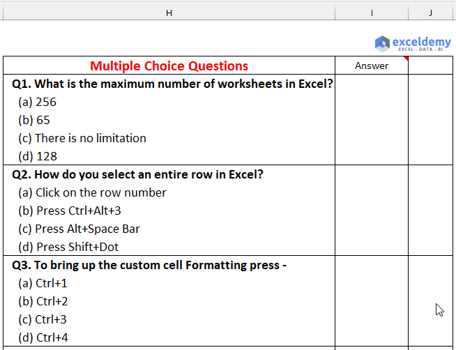
The following animated image shows how to input the answer in the “Problem” sheet. Here, we have typed the answer to the 100 MCQ Excel, but you can use the dropdown list to do so.

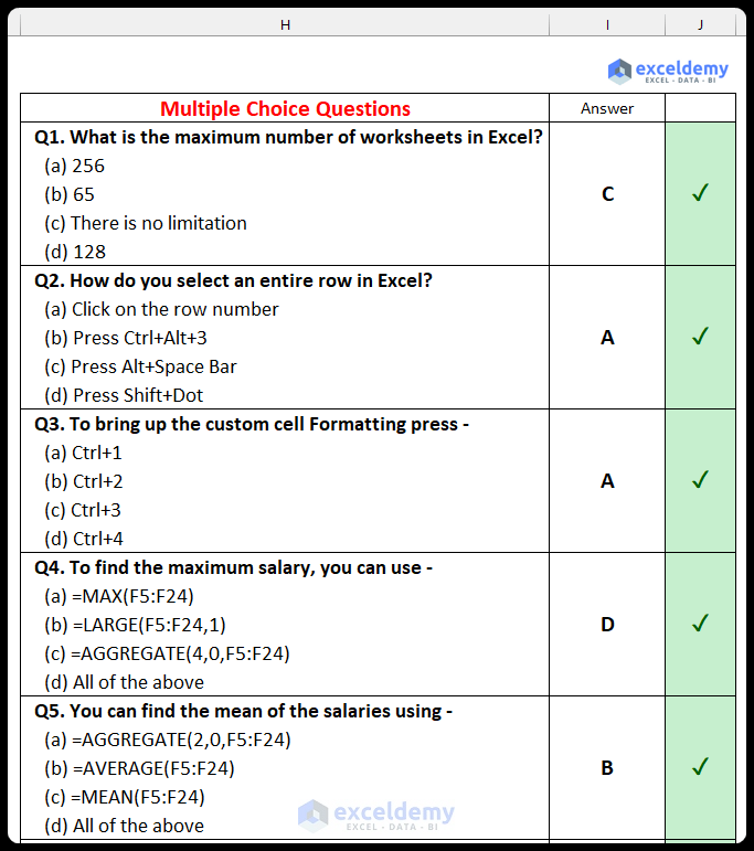
Lastly, the image below shows the “Solution” sheet, which contains the answers to the top 100 MCQs of Excel.

Download Practice Workbook

Conclusion

Thank you for reading this article. By completing this article, we hope that you have gained knowledge about the top 100 MCQ of Excel and their answers. You can find more articles similar to the 100 MCQ Excel on the ExcelDemy website. If you have any questions or suggestions regarding the top 100 MCQ Excel, feel free to comment below. However, remember that our website implements comment moderation. Therefore, your comment may not be instantly visible. So, have a little bit of patience, and we will solve your query as soon as possible. Keep excelling!