You will do all your work in a workbook file. You can add as many worksheets as you need in a workbook file. Each worksheet appears in its own window. By default, Excel workbooks use a .xlsx file extension. This article will assist you in understanding Excel spreadsheets.
Create a new workbook file on your working device. Give it a name, whatever you like. Mine is named “Understanding Spreadsheets.xlsx.” Read the next section for Understanding Excel Spreadsheets.
Understanding Excel Spreadsheets: 29 Common Aspects
You will find 29 options in this article that will boost your foundation of understanding of Excel spreadsheets. You will learn how to create an Excel file, navigate through the file, use some keyboard shortcuts, enable the Quick Access toolbar, view the properties of a spreadsheet, etc.
1. Creating an Excel Workbook from an Existing Excel File
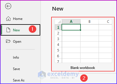
Before describing the elements for understanding Excel spreadsheets, let’s see how you can create one. Say you have an existing workbook file and it is open now. Then just go to File and click New and then click ‘Blank workbook‘.
- The command is File ⇒ New ⇒ Blank workbook. Observe the image below.
2. Creating New Excel Workbook
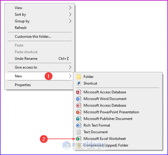
You can create a new workbook file by just clicking the right button of your mouse in a folder. Right-click will generate a shortcut menu.
- You will select “New,” and this will pop up some options.
- From the options, you will click “Microsoft Excel Worksheet”. See the image below.
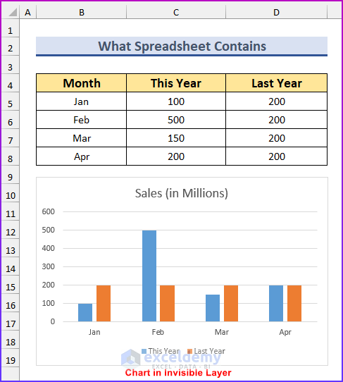
3. What Spreadsheets Contain
Every workbook contains one or more worksheets, typically called spreadsheets. You can add as many worksheets as you need to a workbook. Worksheets are made up of cells. Cells can contain numeric values, formulas, or texts. A worksheet also has an invisible draw layer. This layer holds charts, images, and diagrams.
Read More: How to Create Multiple Sheets in Excel at Once
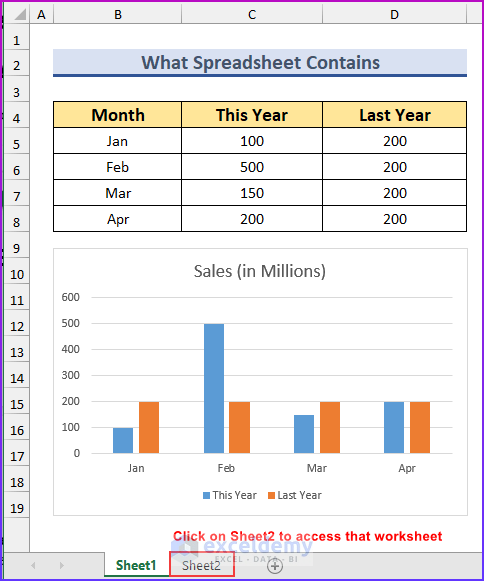
4. Accessing Excel Worksheets
You can access each worksheet by clicking the tabs at the bottom of the workbook window. By default, the font color of the active sheet is Green.
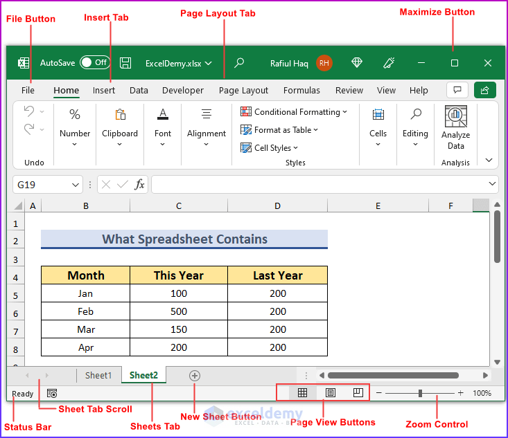
5. Excel Window Elements
It is very important to be familiar with Excel’s windows. If you are a new learner of Excel, it may take some time, but after some days you will feel at home. Every Microsoft product is user-friendly. A layman can use them. Excel is the same.
- In the following image, we have annotated the
- “File Button”
- “Insert Tab”
- “Page Layout Tab”
- “Maximize Button”
- “Status Bar”
- “Sheet Tab Scroll”
- “Sheets Tab”
- “New Sheet Button”
- “Page View Buttons”
- “Zoom Control”
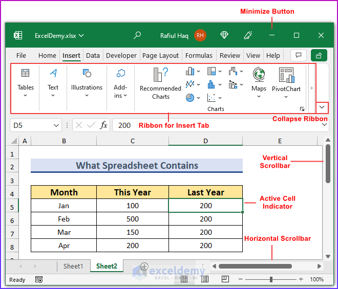
- Again in another snapshot, we’ve marked the following things:
- “Minimize Button”
- “Collapse Ribbon Button”
- “Ribbon for Insert Tab”
- “Vertical Scrollbar”
- “Active Cell Indicator”
- “Horizontal Scrollbar”
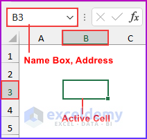
6. Active Cell Indicator of Excel Spreadsheets
The dark outline indicates that this cell is active now. If you input something through the keyboard, the input will be entered in the active cell.
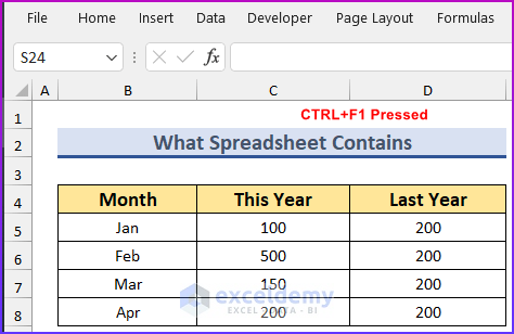
7. Collapse Ribbon (CTRL+F1) Option in Excel Spreadsheets
If you click on “Full-screen mode” or “Show tabs only”, Ribbon will temporarily hide. Alternatively, you can press CTRL+F1 to do so.
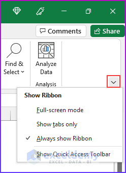
8. Showing Ribbon Option for Excel Spreadsheets
To show the Ribbon again, you have to click Ribbon Display Options and select Show Tabs and Commands. See the images below.
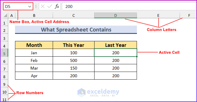
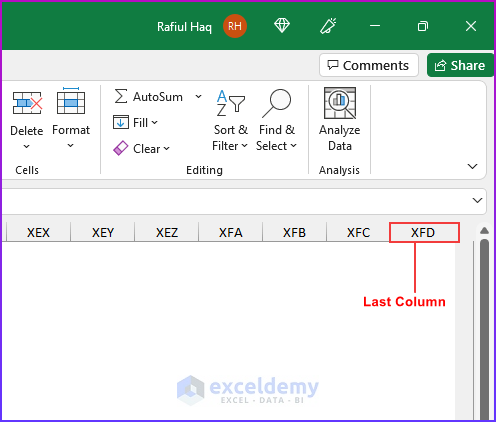
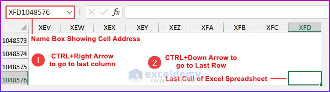
9. Column Letters of Excel Spreadsheets
Letters range from A to XFD. So there are a total of 16,384 columns in a worksheet. See the following image to see the XFD column in the worksheet. If you want to find the XFD column, you have to click and hold your mouse wheel and move the mouse right until you reach the XFD column.
- The keyboard shortcut to find the last column is: End+Right Arrow(→).
- Alternatively, CTRL+Right Arrow will do so too.
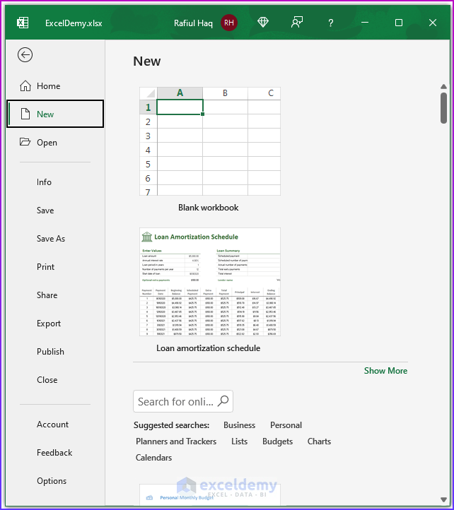
10. File Button for Excel Spreadsheets
If you click the File button, you will see the backstage screen of Excel 365. The backstage screen has many options. The options are Info, New, Open, Save, Save As, Print, Share, Export, Close, Account, and Options.
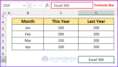
11. Formula Bar for Excel Spreadsheets
When you enter something (a numeric value/ formula/ text) in an active cell, the data is shown in the Formula Bar. See the image below. Here, the Formula Bar is showing a text.
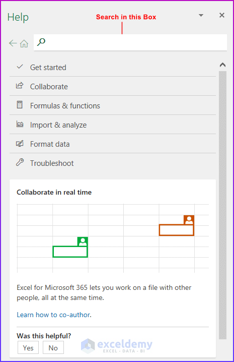
12. Help Button of Excel Spreadsheets
Click the Help button to display the Excel Help system window. Alternatively, you can press F1 to display it.
- If you click on Get Started, you will get a help article titled “Create a workbook in Excel”.
- The other available options are:
- “Collaborate”
- “Formulas & functions”
- “Import & analyze”
- “Format data”
- “Troubleshoot”
13. Horizontal Scrollbar of Excel Spreadsheets
With the Horizontal Scrollbar, you can scroll the worksheet horizontally. There are other options with this scrollbar. Right-click on the horizontal bar, and you will see the following options. See the image below.
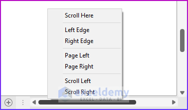
- Left Edge: If you choose this option, the scrollbar will be on the left side of the scroll field.
- Right Edge: If you choose this option, the scrollbar will be on the right side of the scroll field.
- Page Left: If you choose this option, the worksheet will travel one full window left.
- Page Right: If you choose this option, the worksheet will travel one full window right.
- Scroll Left: If you choose this option, the worksheet will travel one column left.
- Scroll Right: If you choose this option, the worksheet will travel one column right.
Note: Whether you use a vertical scrollbar or horizontal scrollbar, your worksheet will move, but there will be no change in active cell selection.
Read More: How to Create Multiple Sheets with Same Format in Excel
14. Name Box of Excel Spreadsheets
The name box shows the address of the active cell. The letter part of the address comes from column letters, and the number part comes from row numbers. B3 means the active cell is now in the B column and third row.
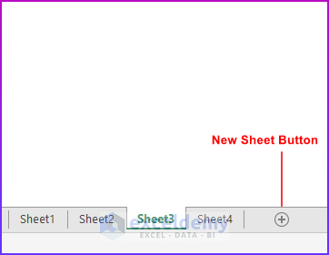
15. New Sheet Button of Excel Spreadsheets
When you want to create a new Excel worksheet, click this button. A new sheet is placed after the last sheet tab. See the image below.
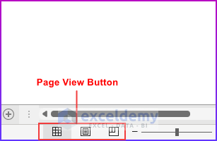
16. Page View Buttons of Excel Spreadsheets
You can change the display views of the worksheets by clicking these three options. Three options are Normal, Page Layout, and Page Break Preview.
Read More: How to Create Multiple Sheets in Excel with Different Names
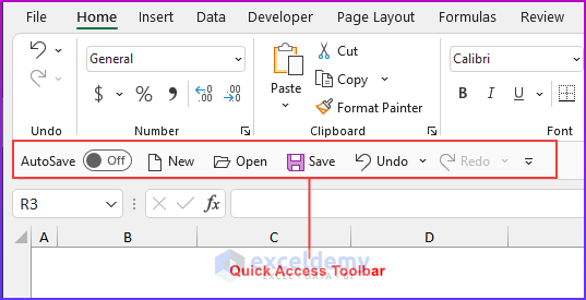
17. Quick Access Toolbar of Excel Spreadsheets
This customizable toolbar holds commonly used commands. Whatever tab (Home/Insert/Page Layout/Formulas/others) you are using, this toolbar is always visible.
- You can add more commands to this toolbar from File → Options → Quick Access Toolbar.
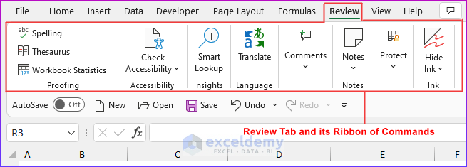
18. Ribbon of Excel Spreadsheets
The ribbon contains the maximum number of commands. When you select Home from the tab list, a ribbon for Home is shown. When you select the Insert tab from the tab lists, a ribbon for Insert is shown. You select commands from Ribbon to work with. The following image shows the ribbon for the Review tab.
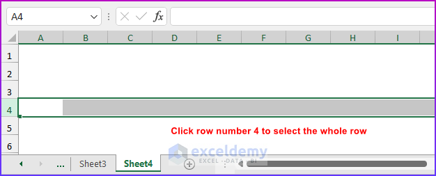
19. Row Numbers of Excel Spreadsheets
Numbers range from 1 to 10,48,576. If you click a row number, then you will select all the cells in that row. If you want to find the 10,48,576th row, you have to click and hold your mouse wheel and move the mouse down until you reach the 10,48,576th row. It will take a long time, so don’t try it. Use keyboard shortcuts.
- The keyboard shortcut to find the last row is End+Down Arrow(↓).
- Alternatively, you can press CTRL+Down Arrow to do so. In the below image, the last cell address is shown.
- Moreover, selecting the row number will select the whole row.
20. Sheet Tabs of Excel Spreadsheets
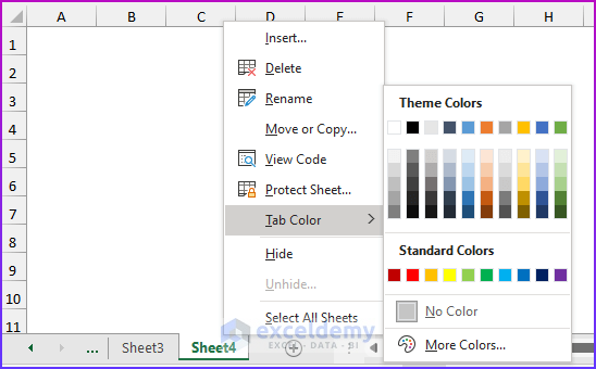
By default, sheet tabs are named ‘Sheet1’, ‘Sheet2’, and so on. A workbook can have any number of sheets and each sheet has its name displayed in the sheet tab. If you right-click on a sheet tab, you will have many options to apply to the sheet tab. See the image below.
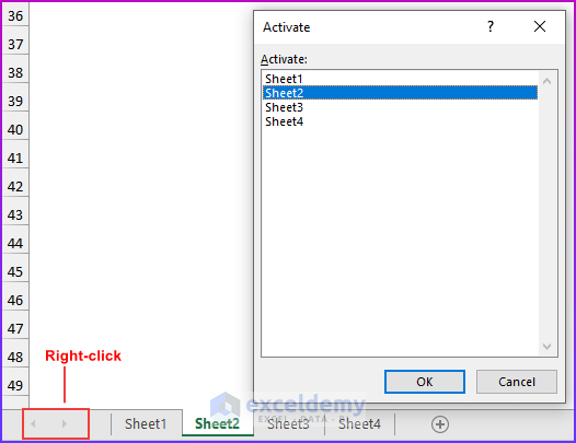
21. Sheet Tab Scroll Buttons of Excel Spreadsheets
You will use these buttons to scroll the sheet tabs to display tabs that aren’t visible. You can also right-click to get a list of sheets. See the image below.
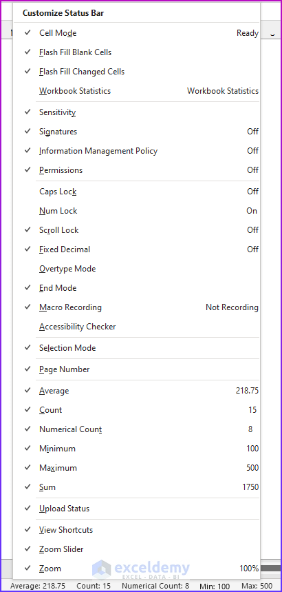
22. Status Bar of Excel Spreadsheets
The status bar displays various statuses, including the status of the Num Lock, Caps Lock, and Scroll Lock keys on your keyboard. If you select a range of cells in your worksheet, it will show you summary information about the cells you have selected.
- For example, when you select the cell range B4:D8, you will see various calculations for that range.
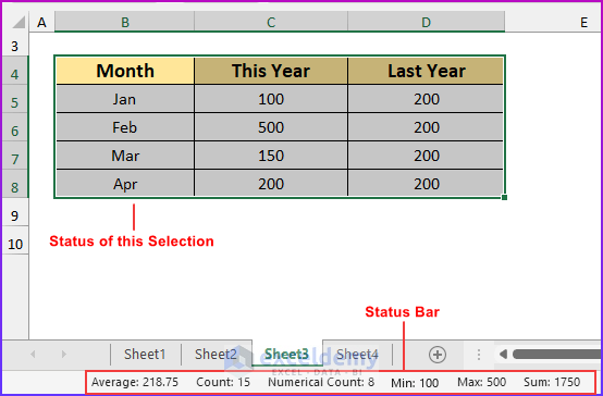
- Just right-click on the Status Bar and select which information you want to see in the Status Bar.
23. Tab List of Excel Spreadsheets
By default, we see Home, Insert, Data, Developer, Page Layout, Formulas, Review, View, Help, and these 9 tab names in the tab list. You can customize the ribbon. Click on these tab names and you will see that every tab has its own ribbon. The tab is similar to the Menu.
- Here we see the tab Review is selected, and the ribbon is showing the commands of the Review tab.
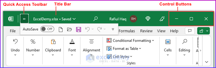
24. Title Bar of Excel Spreadsheets
The title bar shows the name of the program (the program is Excel) and the name of your workbook. It also holds the Quick Access toolbar (on the left) and some control buttons that you will use to modify the window (on the right).
- The Quick Access Toolbar can be shown below the Ribbon.
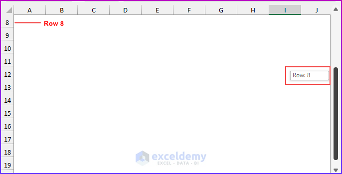
25. Vertical Scrollbar of Excel Spreadsheets
You will use this scrollbar to scroll your worksheet vertically. If you drag the scrollbar, you will see the row number, and this row number is the first row of your worksheet.
Right-click on the vertical scrollbar. You will receive some option commands. See the image below.
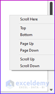
- Top: If you choose this option, the scrollbar will be at the top of the scroll field.
- Bottom: If you choose this option, the scrollbar will be at the bottom of the scroll field.
- Page Up: If you choose this option, the worksheet will travel one full window up.
- Page Down: If you choose this option, the worksheet will travel one full window down.
- Scroll Up: If you choose this option, the worksheet will travel one column up.
- Scroll Down: If you choose this option, the worksheet will travel one column down.
Note: Whether you use a vertical scrollbar or a horizontal scrollbar, your worksheet will move, but there will be no change in the Active Cell selection.
Read More: How to Create New Sheets for Each Row in Excel
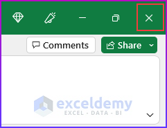
26. Window Close Button in Excel Spreadsheets
Click this button to close the active workbook window. If you have not saved your workbook, then Excel will ask you to save the file.
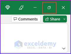
27. Window Maximize/Restore Button for Excel Spreadsheets
Click this button to increase the workbook window’s size to fill your entire computer screen. If the window is already maximized, clicking this button will reduce Excel’s window so that it no longer fills the entire screen.
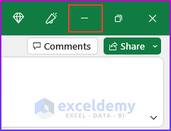
28. Window Minimize Button in Excel Spreadsheets
Click this button to minimize the workbook window. The window displays as an icon on your Windows Taskbar.
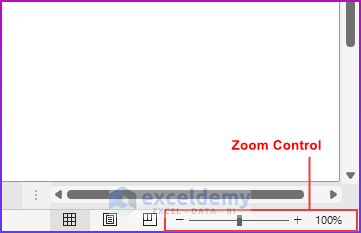
29. Zoom Control
Use this to zoom your worksheet in and out. You can zoom out to view a large dataset, or you can zoom in to observe a smaller dataset with ease. This will be the last and final topic for understanding the Excel spreadsheet environment.
Download Practice Workbook
Conclusion
We wanted to cover the basic stuff about understanding Excel spreadsheets. If you face any problems, feel free to comment below and our team will get back to you as soon as possible.
Related Articles
- How to Create Multiple Worksheets from a List of Cell Values
- How to Insert Sheet from Another File in Excel
<< Go Back to Insert Sheet | Worksheets | Learn Excel
Get FREE Advanced Excel Exercises with Solutions!
