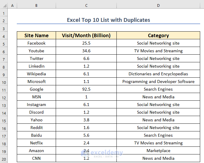
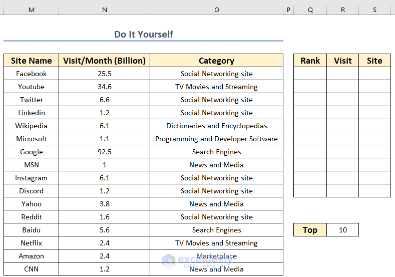
Below is a basic table listing the sites and their respective monthly visits. The second column has a couple of duplicate values.
Method 1 – Incorporating LARGE Function with the INDEX–MATCH Formula
Steps:
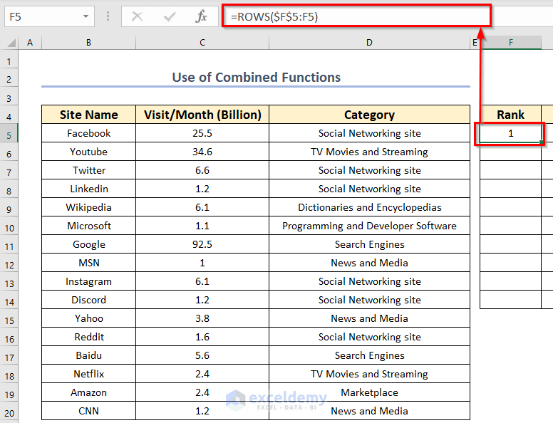
- Select a new cell, F5, where you want to keep the result.
- Enter the formula given below in cell F5:
=ROWS($F$5:F5)Here, the ROWS function will give the relative row number from a given array.
- Press ENTER.
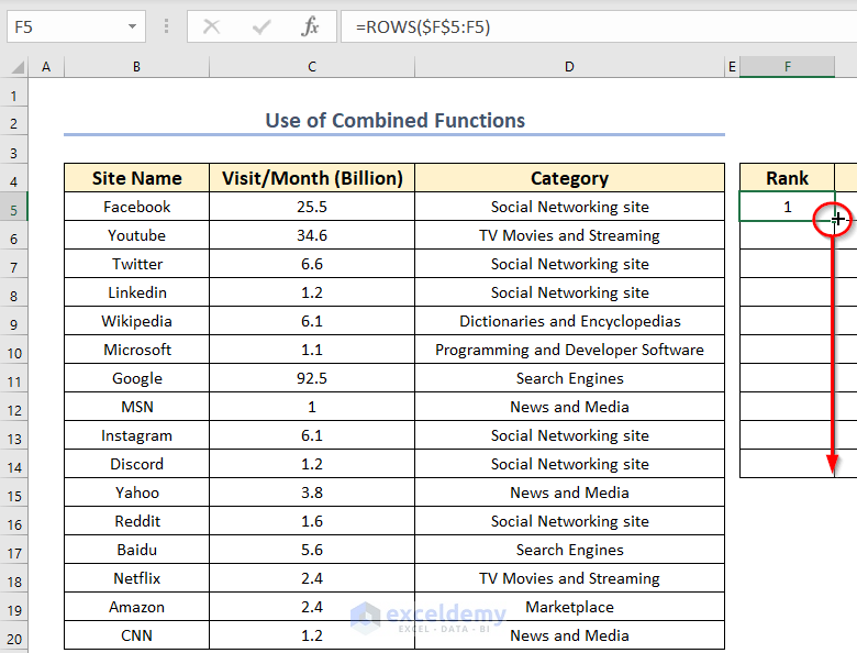
- Drag the Fill Handle icon to AutoFill the corresponding data in the rest of the cells F6:F14.
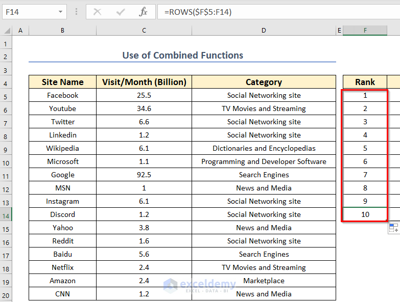
As a result, you will see the rank.
To do the task, we need to use the LARGE function. The LARGE function returns numeric values based on their position in a list when sorted by value.
array: The array from which you want to select the kth largest value.
k: An integer that specifies the position from the largest value.
Here, we will provide the position using the k. When we need the top 10 value, then the value of k will be 1 to 10.
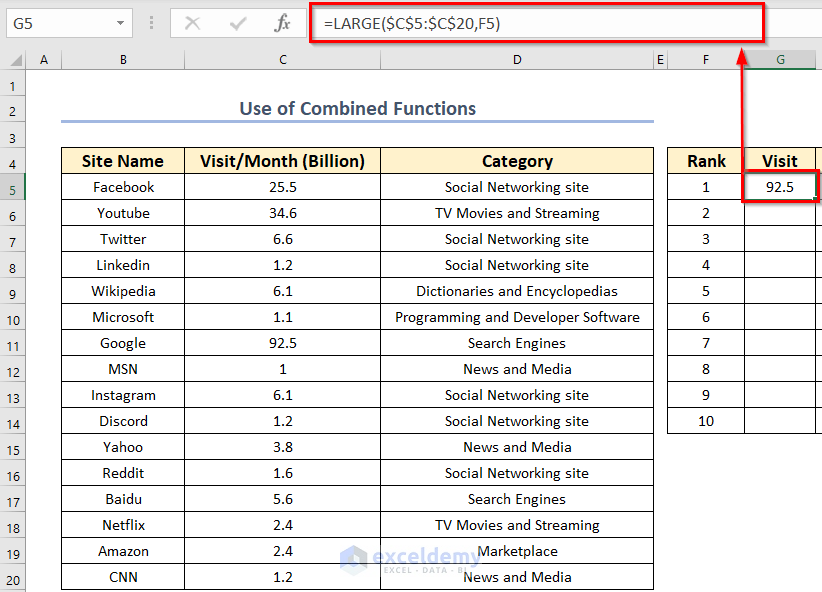
- Select a new cell, G5, where you want to keep the result.
- Enter the formula below in cell G5:
=LARGE($C$5:$C$20,F5)- Press ENTER.
We have inserted the visits amount column as the array and the Rank as the k.
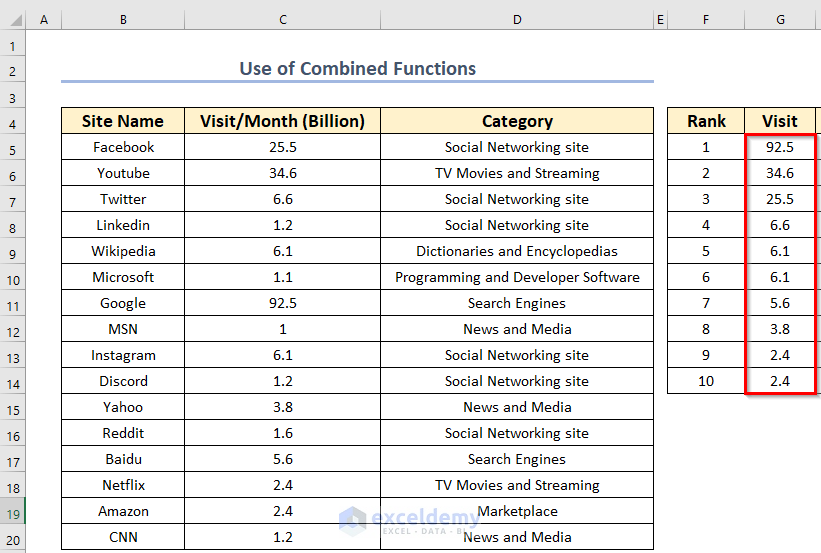
- Enter the formula for the rest.
We have found the top 10 most visited sites from our list.
To find the names, we need to use the combination of the INDEX–MATCH functions.
Here, the MATCH function is used to locate the position of a lookup value in a row, column, or table.
Additionally, the INDEX function returns the value at a given location in a range or array.
- Enter the following formula in cell H5:
=INDEX($B$5:$B$20,MATCH(G5,$C$5:$C$20,0))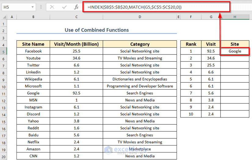
Formula Breakdown
- Firstly, inside the INDEX function, we have inserted the Site Name column as our find_array.
- Secondly, the MATCH function is used to declare the row number.
- Here, within the MATCH function, we have inserted the lookup_value and lookup_array. Our lookup_value is the visit value we have derived. 0 for stating the Exact Match.
- Press ENTER to get the result.
- Enter the formula for the rest of the rows.
Oh! Not the items we were looking for.
Our table has several duplicate visits. Here, a couple of sites have the same number of visits. Our formula should derive both names, but this formula is unable to do that.
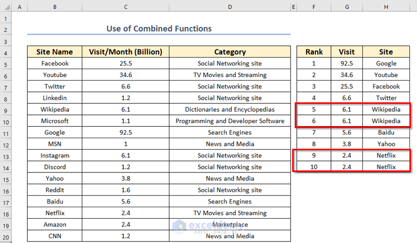
We need to modify the formula.
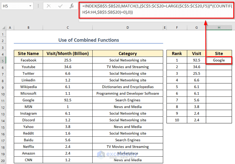
- Our modified formula will be as follows:
- Enter the formula in cell H5:
=INDEX($B$5:$B$20,MATCH(1,($C$5:$C$20=LARGE($C$5:$C$20,F5))*(COUNTIF(H$4:H4,$B$5:$B$20)=0),0))- Press ENTER.
Formula Breakdown
- Here, in the MATCH function, we have set 1 as the lookup_value.
- Then we compared the value using $B$4:$B$19=LARGE( $B$4:$B$19, E4). This will return an array of TRUE or FALSE.
- Now, the COUNTIF function, with an expanding range of references, checks if a given item is already in the top list and returns an array of TRUE or FALSE.
- After that, when we multiply these two arrays, another array of 1s and 0s is returned.
- Here, the lookup_value 1 matches this array and returns the relative position.
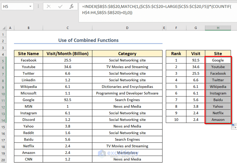
- Enter the formula for the rest of the rows.
Read More: How to Get Top 10 Values Based on Criteria in Excel
Method 2 – Using a Combination of SMALL and INDEX Functions
Steps:
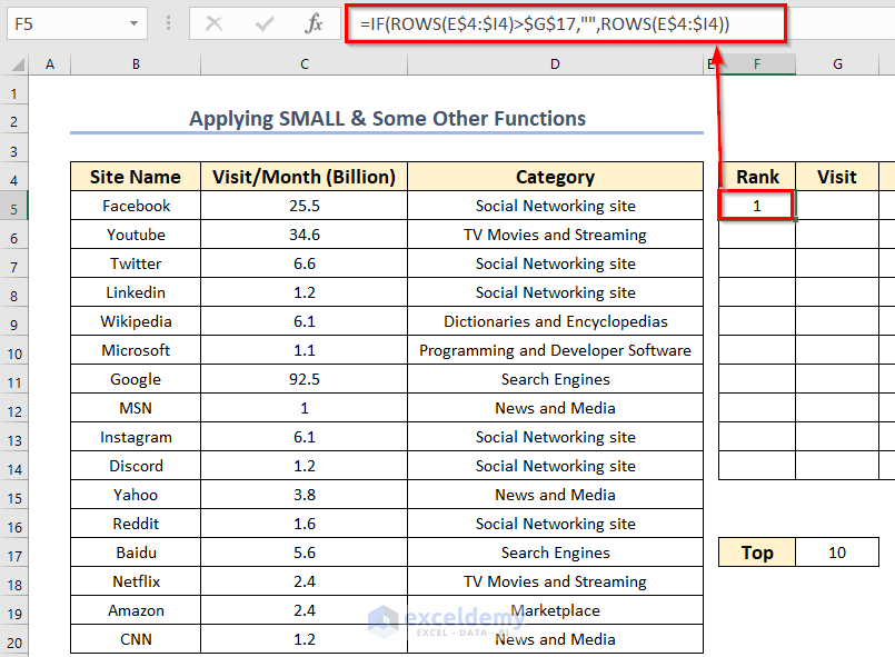
- Enter the IF function in cell F5.
=IF(ROWS(E$4:$I4)>$G$17,"",ROWS(E$4:$I4))- Press ENTER.
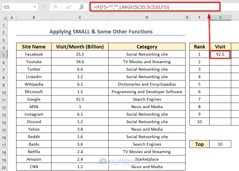
- Enter the following formula in cell G5:
=IF(F5="","",LARGE($C$5:$C$20,F5))- Press ENTER.
Our formula to find the items will be as follows:
- Use the IF statement as previously to eradicate any error for the empty cells.
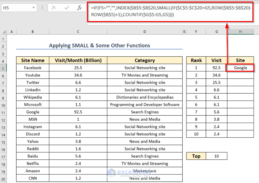
- Enter the following formula in cell H5:
=IF(F5="","",INDEX($B$5:$B$20,SMALL(IF($C$5:$C$20=G5,ROW($B$5:$B$20)-ROW($B$5)+1),COUNTIF($G$5:G5,G5))))- Press ENTER to execute the formula.
Formula Breakdown
- Here, we find the row_number for the INDEX function using the SMALL function.
- Then, inside the SMALL function, we have an IF function that checks whether the lookup_value is within the array.
- Furthermore, the ROW functions generate the row numbers starting from 1.
- In addition, the COUNTIF function is for checking whether the value has already been traversed or not.
- Lastly, the combination of the result from these functions produces a row_number that must be fetched from the array.
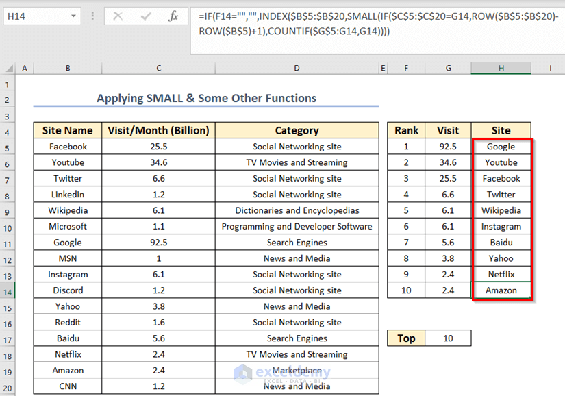
We have found the Site name that topped the list.
- Enter the formula or exercise Excel AutoFill for the rest of the values.
Method 3 – Using the AGGREGATE Function
Steps:
- Enter the formula for Rank and Visit column like the previous method.
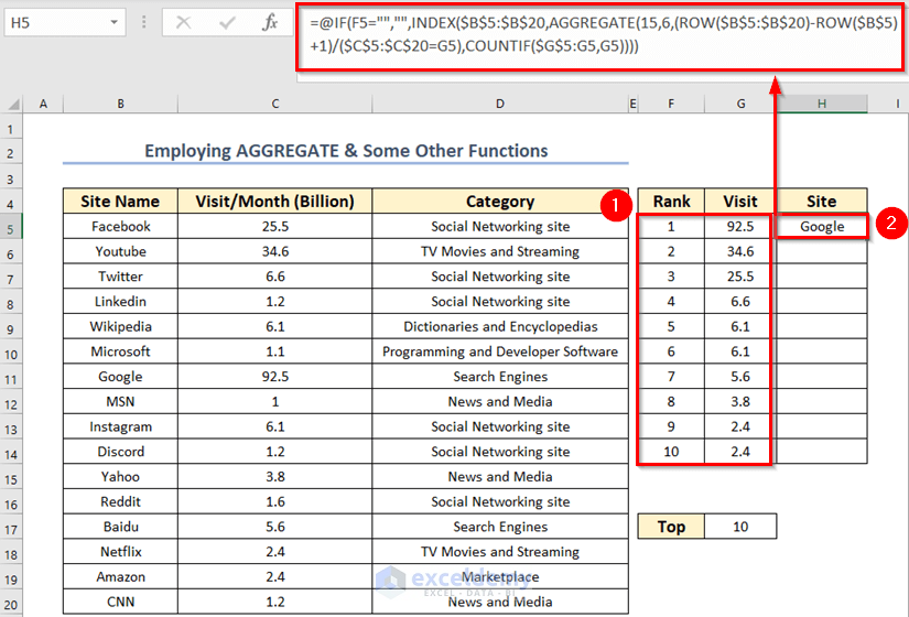
- Enter the following formula in cell H5:
=@IF(F5="","",INDEX($B$5:$B$20,AGGREGATE(15,6,(ROW($B$5:$B$20)-ROW($B$5)+1)/($C$5:$C$20=G5),COUNTIF($G$5:G5,G5))))- Press Enter.
- Enter the ROW function division portion in Excel. As a result, a bunch of division errors within the array.
- To ignore the error, we have used 6 as our behavior_option value.
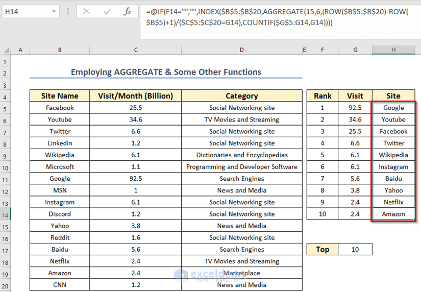
- Enter the formula for the rest of the rows, and you will get the top 10 from the list with duplicates.
Method 4 – Using FILTER & SORT Functions
Steps:
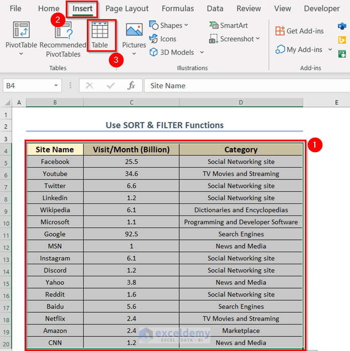
- Select the data range.
- From the Insert tab >> choose the Table feature.
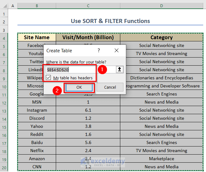
A dialog box named Create Table will appear.
- Select the data range in the Where is the data for your table? box. If you select the data range before, this box will auto-fill.
- Check the My table has headers option.
- Press OK.
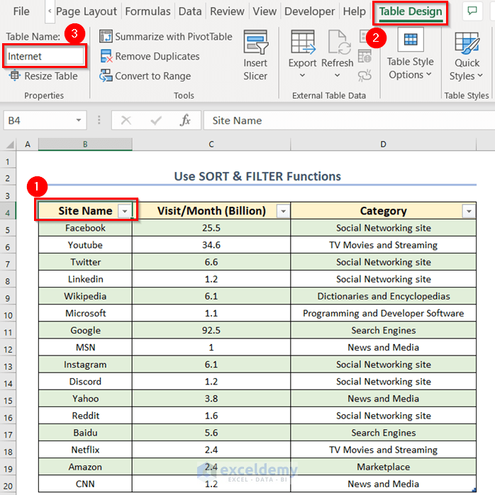
Your table is ready.
- Select any cell of the table.
- From the Table Design tab >> go to the Properties option.
- Enter a table name in the Table Name box. Here, we have written Internet as the table name.
- Select a different cell with enough space to keep all your data.
- Enter the following formula in that cell. Here, we’re going to use cell F8.
=IF(COUNT((Internet[Visit/Month (Billion)]))>H5,SEQUENCE(H5),"Cross Limit")- Press ENTER to get the result.
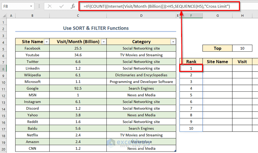
Formula Breakdown
- Here, the COUNT function will count the total cells of Internet[Visit/Month (Billion)]) column.
- Then, the IF function will check whether the number of counted cells is greater than the H5 cell value.
- If the H5 cell value is less than the total counted cells, it will operate the SEQUENCE function; otherwise, it will return “Cross Limit”.
- Select a different cell with enough space to keep all your data.
- Enter the following formula in that cell. Here, we’re going to use cell G8.
=SORT(FILTER(Internet,Internet[Visit/Month (Billion)]>=LARGE(Internet[Visit/Month (Billion)],H5)),2,-1)- Press ENTER.
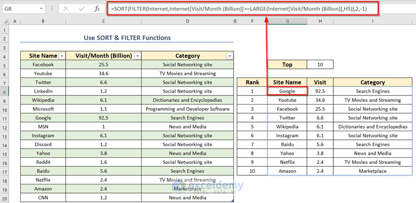
Formula Breakdown
- Here, the H5 cell will be the search box.
- Firstly, the LARGE function will return the 10th large value from the column Internet[Visit/Month (Billion)].
- Output: 2.4.
- Secondly, the FILTER function will filter the data. Here, the array is a table named Internat. It will search for values greater than or equal to 2.4 and return all the details of the Visit value, like Site Name—Visit—Category.
- Output: {“Facebook”,25.5,”Social Networking site”;”Youtube”,34.6,”TV Movies and Streaming”;”Twitter”,6.6,”Social Networking site”;”Wikipedia”,6.1,”Dictionaries and Encyclopedias”;”Google”,92.5,”Search Engines”;”Instagram”,6.1,”Social Networking site”;”Yahoo”,3.8,”News and Media”;”Baidu”,5.6,”Search Engines”;”Netflix”,2.4,”TV Movies and Streaming”;”Amazon”,2.4,”Marketplace”}.
- Thirdly, 2 is the sort index, and -1 is the sort order for the SORT function. So, the SORT function will sort the Visit/Month (Billion) column in descending order.
You will get the top 10 list.
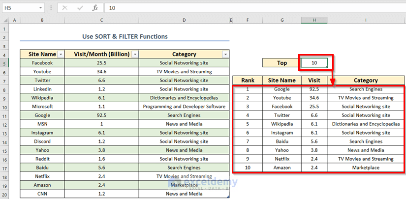
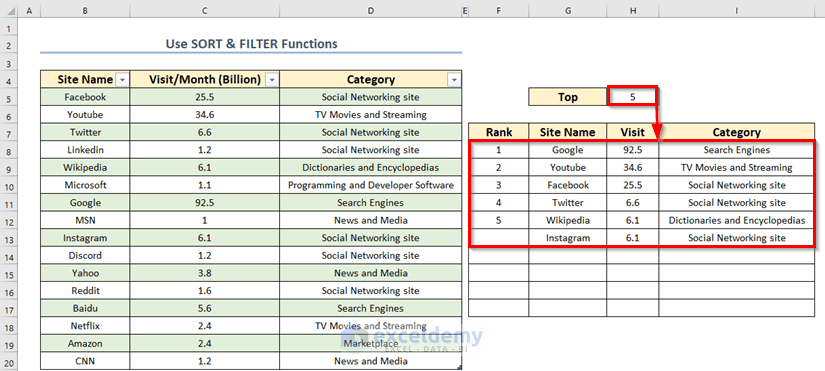
If you want to know the top 5 list with duplicates, write 5 in cell H5. The result will be auto-modified.
Read More: How to Find Top 5 Values and Names in Excel
Method 5 – Inserting a Pivot Table
Steps:
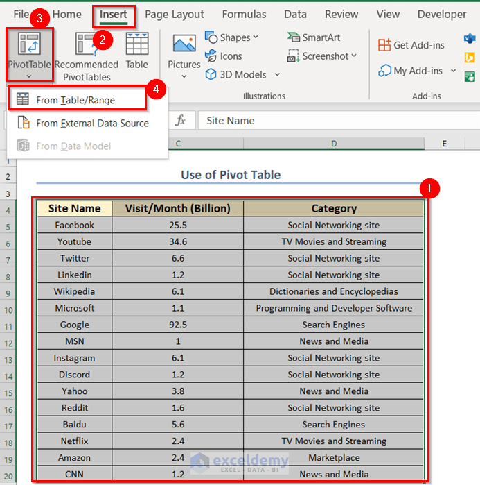
- Select the entire table and then explore the Insert tab, you will find the Tables section.
- In the Tables section, Click Pivot Table.
- Choose the From Table/Range option.
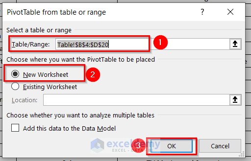
A dialog box will open.
- Check the range and select the place.
- Click OK
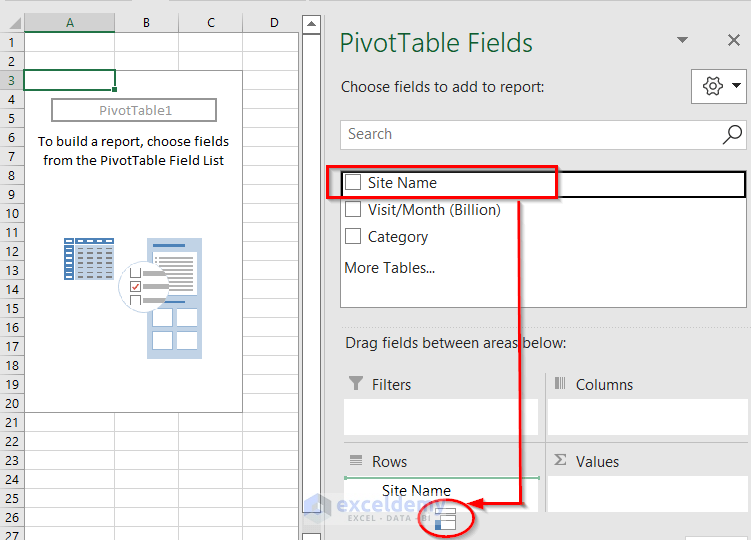
A new sheet will open like the following image.
- Drag the Site Name to the Rows.
You will see the Row Labels.
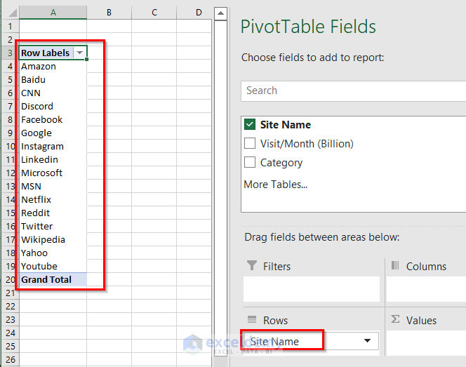
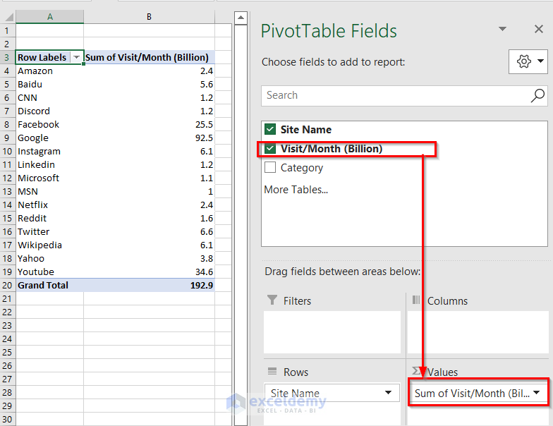
- Drag the Visit column to the Values.
The Pivot Table sums up the numeric values.
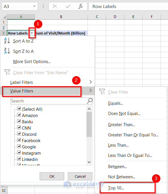
- Click the Filter icon beside the Row Labels.
- In the Value Filters, you will find the Top 10 option. Click that.
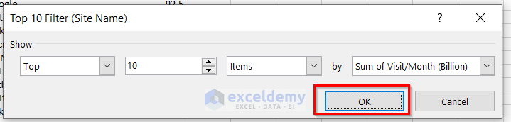
A dialog box will pop up.
- Click OK.
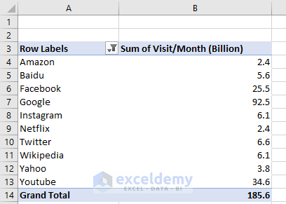
You will find the top 10 values from your list.
Practice Section
You can practice the methods here.
Download the Practice Workbook
Download the workbook to practice.
Related Articles
- How to Check If a Value is in List in Excel
- Lookup Value in Column and Return Value of Another Column in Excel
- Find Text in Excel Range and Return Cell Reference
- How to Search Text in Multiple Excel Files
- [Solved!] CTRL+F Not Working in Excel
<< Go Back to Find Value in Range | Excel Range | Learn Excel
Get FREE Advanced Excel Exercises with Solutions!

Hello,
all these functions not working with WPC Office, tried everything, i miss something? Therefore these functions
work only in Microsoft 365?
Thank you!
Dear Andrei,
These functions are available in WPS office.
Regards
ExcelDemy