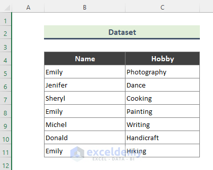
We have a dataset containing the hobbies of several people. However, one person (Emily) has more than one hobby. We will show how you can extract multiple values with this dataset as an example.
Method 1 – Using Find and Replace to Get Multiple Values in Excel
Steps:
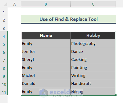
- Select the dataset (B4:C11).
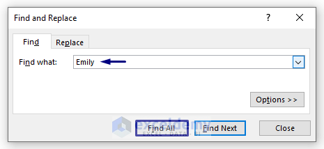
- Press Ctrl + F to bring up the Find and Replace window or go to Home and select Find & Select, then click on Find.
- Type Emily in the Find what field and click on Find All.
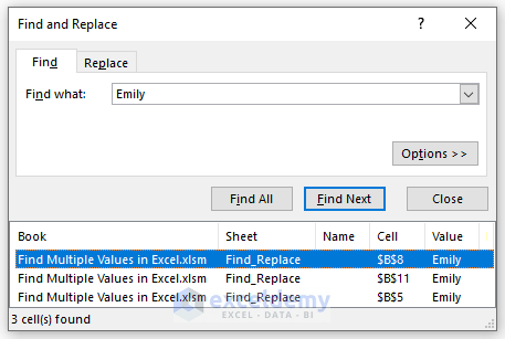
- The dialog will display 3 cells that contain the string Emily below.
Method 2 – Applying the Filter Option to Find Multiple Values
Steps:
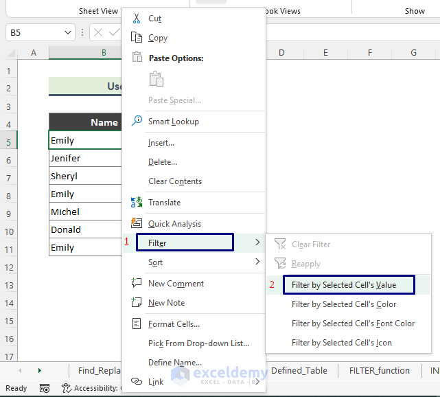
- Right-click on the cell to which you want to apply the filter. We have selected Cell B5, as we need to filter by the name Emily.
- Go to Filter and select Filter by Selected Cell’s Value.
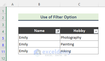
- All the cells containing the name Emily are filtered as below.
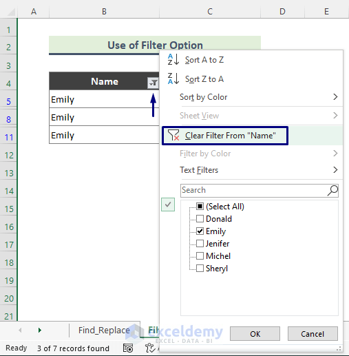
- If you want to undo the filtering, click on the Autofilter icon of the dataset header then select Clear Filter From “Name” and click OK.
Method 3 – Utilizing the Advanced Filter to Return Multiple Values
Steps:
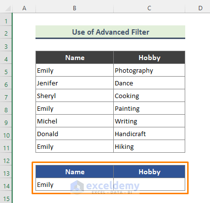
- Set the criteria range (B13:C14).
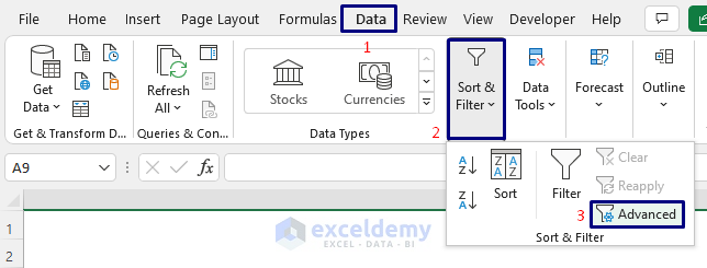
- Go to Data and choose Sort & Filter, then select Advanced.
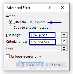
- The Advanced Filter window will show up. Set the List range (Dataset range) and Criteria range, then click OK.
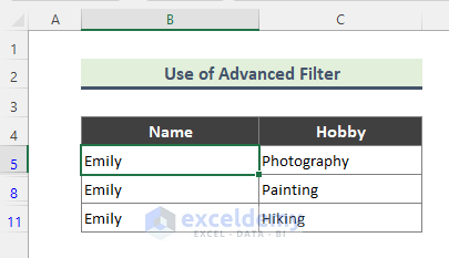
- We got all of Emily’s hobbies at once.
Remember, the Header of the main dataset and the Criteria range have to match or the Advanced Filter option will not work.
Method 4 – Returning Multiple Values by Using a Defined Table
Steps:
- Click on any of the cells of the dataset (B4:C11).
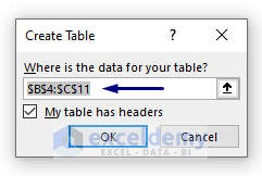
- Press Ctrl + T from the keyboard. The Create Table window will show up.
- Check the table range and click OK.
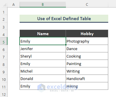
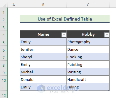
- You’ll get a table created from the dataset.
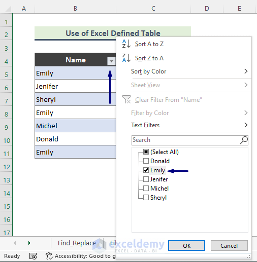
- Click on the down arrow icon next to the header of the table.
- Check the name Emily and click OK
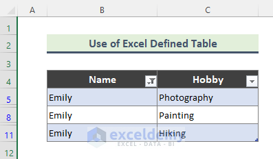
- Here is our expected filtered result.
Method 5 – Inserting the FILTER Function to Find Multiple Values
Steps:
- Use the following formula in cell C14.
=FILTER(C5:C11,B5:B11=B14)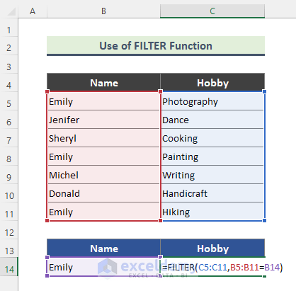
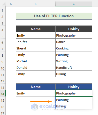
- Hit Enter.
- All of Emily’s hobbies will be listed.
Note: The FILTER function is only available for Excel 365.
Method 6 – Searching Multiple Values with the INDEX Function in Excel
Steps:
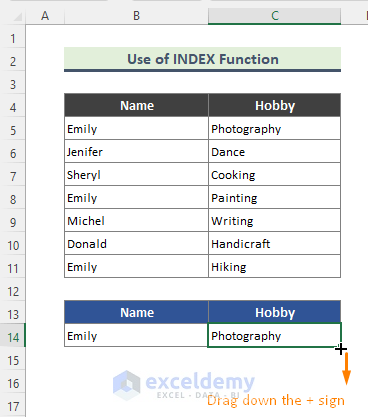
- Use the following formula in Cell C14.
=INDEX($B$5:$C$11,SMALL(IF($B$5:$B$11=$B$14,ROW($B$5:$B$11)),ROW(1:1))-4,2) 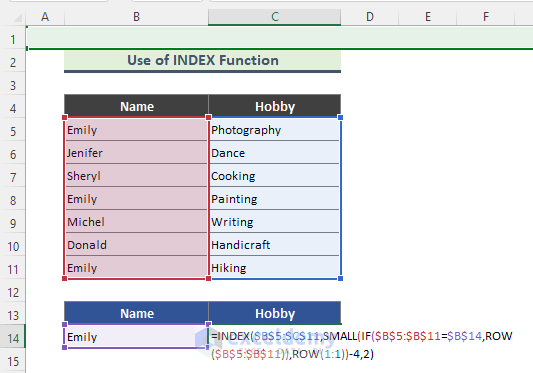
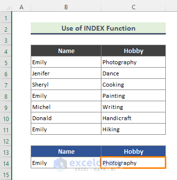
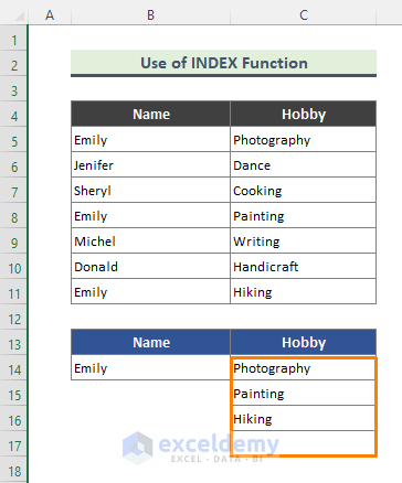
- Here’s our first result.
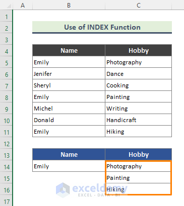
- Drag down the Fill Handle (+) sign to get the other values.
- Here is the list of Emily’s hobbies.
How does the Formula Work?
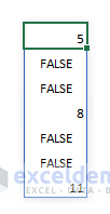
- IF($B$5:$B$11=$B$14,ROW($B$5:$B$11))
The IF function returns a row number if a cell range B5:B11 is equal to B14.
- SMALL(IF($B$5:$B$11=$B$14,ROW($B$5:$B$11)),ROW(1:1))
This part of the formula uses the SMALL function which returns the nth smallest value. This formula will return the numbers: 5,8,11.
- INDEX($B$5:$C$11,SMALL(IF($B$5:$B$11=$B$14,ROW($B$5:$B$11)),ROW(1:1))-4,2)
Now comes the final part of the formula. We know, the INDEX function returns the value at a given position. Another thing is, the INDEX function considers the first row of our table as row 1. As my table dataset starts in row 5, I have subtracted 4 from the ROW value to get the correct row from the dataset. So, for the array B5:C11, row numbers 5,8,11, and column no 2, the INDEX function will provide our desired result
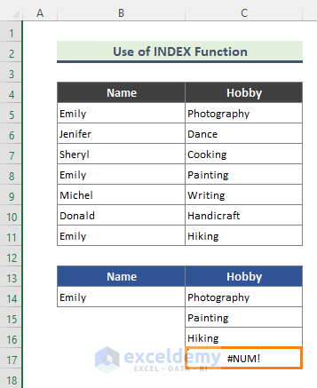
Hide the Errors Generated by the Formula
When you drag down the Fill Handle (+) sign, the formula returns an error (#NUM!) after finding all values.
Steps:
- Use the modified formula in Cell C14.
=IF(ISERROR(INDEX($B$5:$C$11,SMALL(IF($B$5:$B$11=$B$14,ROW($B$5:$B$11)),ROW(1:1))-4,2)),"",INDEX($B$5:$C$11,SMALL(IF($B$5:$B$11=$B$14,ROW($B$5:$B$11)),ROW(1:1))-4,2)) 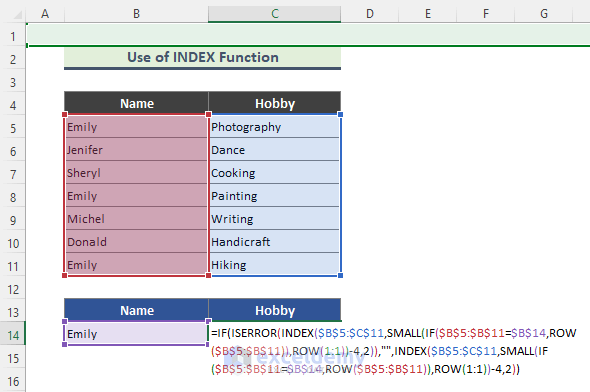
- We won’t get the error values.
The ISERROR function checks whether a value is an error, and returns TRUE or FALSE. The above formula wrapped with IF and ISERROR functions check whether the result of the array is an error or not and thus returns blank (“”) if the result is an error, otherwise, it returns the corresponding value.
Read More: How to Find Value in Column in Excel
Method 7 – Utilizing a User-Defined Function to Find Multiple Values in Excel (VBA)
Steps:
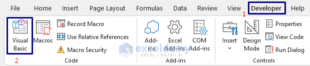
- Go to the active worksheet.
- Go to Developer and select Visual Basic.
- The Visual Basic window will show up. Go to the VBA Project corner (Upper left corner of the window).
- Right-click on the Project name, go to Insert and select Module.
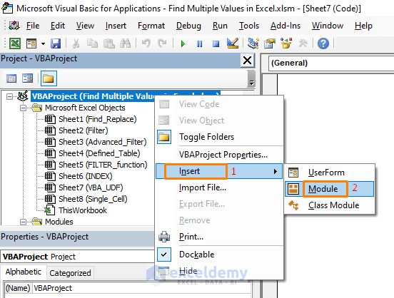
- You will get a Module. Insert the following code in the Module.
'Name User Defined Function and arguments

Function vbaVlookup(lookup_value As Range, tbl As Range, col_index_num As Integer, Optional layout As String = "v")
'Declare variables and data types
Dim r As Single, Lrow, Lcol As Single, temp() As Variant
'Redimension array variable temp
ReDim temp(0)
'Iterate through cells in cell range
For r = 1 To tbl.Rows.Count
   'Check if lookup_value is equal to cell value
   If lookup_value = tbl.Cells(r, 1) Then
      'Save cell value to array variable temp
      temp(UBound(temp)) = tbl.Cells(r, col_index_num)
      'Add another container to array variable temp
      ReDim Preserve temp(UBound(temp) + 1)
   End If
Next r
'Check if variable layout equals h
If layout = "h" Then
   'Save the number of columns the user has entered this User Defined Function in.
   Lcol = Range(Application.Caller.Address).Columns.Count
   'Iterate through each container in array variable temp that won't be populated
   For r = UBound(temp) To Lcol
       'Save a blank to array container
       temp(UBound(temp)) = ""
       'Increase the size of array variable temp with 1
       ReDim Preserve temp(UBound(temp) + 1)
   Next r
   'Decrease the size of array variable temp with 1
   ReDim Preserve temp(UBound(temp) - 1)
   'Return values to worksheet
   vbaVlookup = temp
'These lines will be rund if variable layout is not equal to h
Else
   'Save the number of rows the user has entered this User Defined Function in
   Lrow = Range(Application.Caller.Address).Rows.Count
   'Iterate through empty cells and save nothing to them in order to avoid an error being displayed
   For r = UBound(temp) To Lrow
      temp(UBound(temp)) = ""
      ReDim Preserve temp(UBound(temp) + 1)
   Next r
'Decrease the size of array variable temp with 1
ReDim Preserve temp(UBound(temp) - 1)
'Return temp variable to worksheet with values rearranged vertically
vbaVlookup = Application.Transpose(temp)
End If
End Function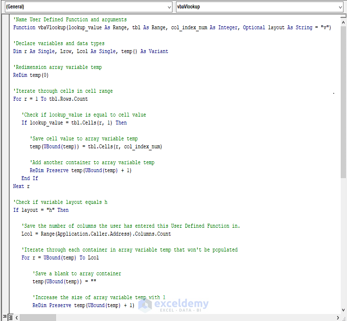
- When you start to write the function name in Cell C14, it will show up like other Excel functions.
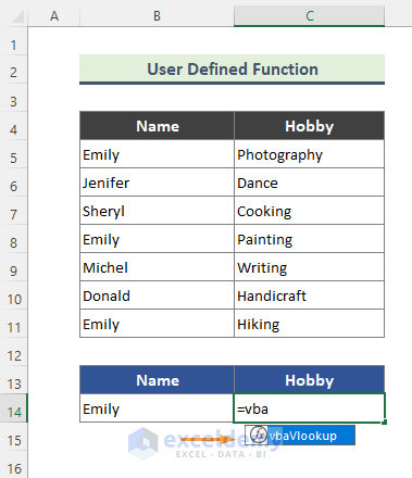
- Insert the following formula in Cell C14.
=vbaVlookup(B14,B5:B11,2)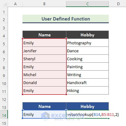
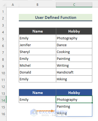
- Here we have multiple hobbies for Emily.
Method 8 – Producing Multiple Values in a Single Cell of Excel
Steps:
- Insert the following formula in Cell C14.
=TEXTJOIN(",",TRUE, FILTER(C5:C11, B5:B11=B14))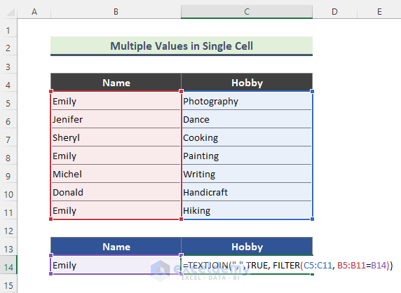
- Here’s the result, with all hobbies listed in a single cell.
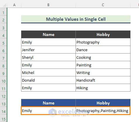
The TEXTJOIN function concatenates the list of hobbies using commas.
Download the Practice Workbook
Further Readings
- How to Find First Value Greater Than in Excel
- How to Find First Occurrence of a Value in a Range in Excel
- Find Last Value in Column Greater than Zero in Excel
- How to Find First Occurrence of a Value in a Column in Excel
- How to Find Last Occurrence of a Value in a Column in Excel
<< Go Back to Find Value in Range | Excel Range | Learn Excel
Get FREE Advanced Excel Exercises with Solutions!

What if I want to find all of the Emily and Jennifers in the set of data at once? I am not finding a way to search for multiple values at once….
Thanks, Janel, for your comment. To find all the data of Emily and Jenifer at once, you can utilize the Filter feature of the Excel table shown in method 4 (Return Multiple Values by Using Excel Defined Table). Here, after clicking the down arrow icon, you need to check both Emily and Jenifer in the filter option to get the hobby list of both persons. Hopefully, it will solve your problem.
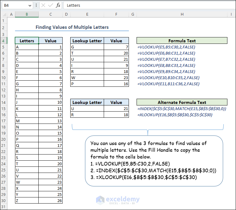
Hello I have a question. Say I have a raw data like: A=1, B=2, C=3, etc. Now I want to find the values of multiple letters, say G T U I R W P. How do I do that?
Hello Saccharine,
Thank you for your query. You can find the answer to your question in the Excel file attached to this message.
How to Find Values of Multiple Letters.xlsx
Here is a sample image of the Excel file.
Hope this helps. Have a good day.
Regards,
Exceldemy
Is it possible to find and delete multiple values at once? Let’s say you had 100 students on the list twice, and you didn’t want to only delete the duplicate names, but also the first ones. Is there a way to do this without searching for each name one-at-a-time?
Hello Amber,
It is possible to find and delete multiple values at once. To delete the first occurrences of duplicate values you can use a helper column to find out those values then apply filter to delete it.
Insert the following formula in a helper column:
=IF(COUNTIF(A2:A12, A2) > 1, IF(COUNTIF(A$2:A2, A2)=1, “Delete”, “Keep”), “Keep”)
It will check the name appears more than once. If it does, it marks the first occurrence with “Delete” and subsequent duplicates with “Keep.” For unique names it will also return “Keep”.
Now, to apply filter to your data from Data tab >> select Filter.
Then select Delete from helper column.
Finally, select all the names and press on Delete.
Download the Excel file:
Remove Duplicates First Occurences.xlsx
Regards
ExcelDemy