Method 1 – XLOOKUP Function to Find Last Occurrence of a Value in a Column
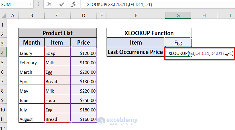
➤Type the following formula in our cell G4.
=XLOOKUP(G3,C4:C11,D4:D11,,,-1)➤ Give lookup_value as G3, lookup_ array as C4:C11, and return_array as D4:D11.
➤ Type “,,,-1” to search from last to first. We’ve skipped several placeholders as we didn’t need those.
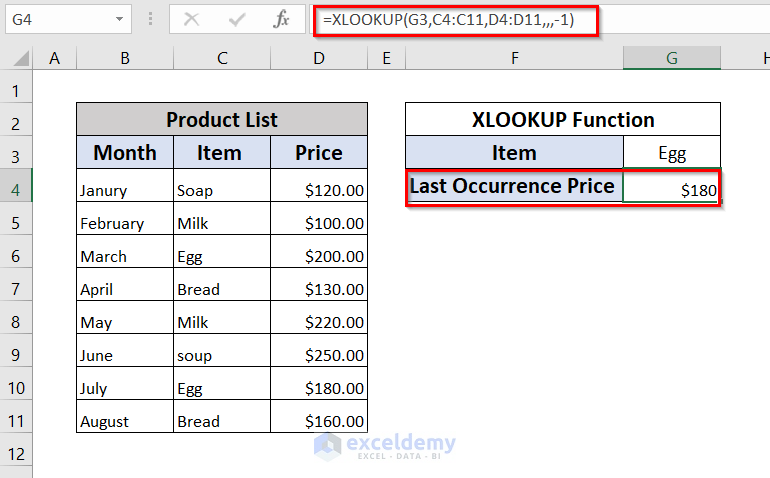
➤Press Enter.
➤We can see the Last Occurrence Price of the Egg is $180, and the formula is in the Formula Bar.
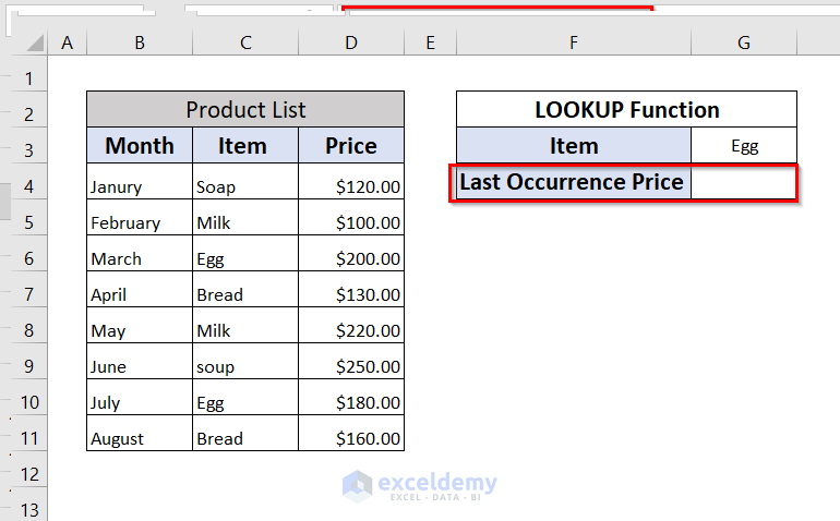
Method-2 – LOOKUP Function to Find Last Occurrence of a Value
Find the Last Occurrence Price of Egg using the LOOKUP function.
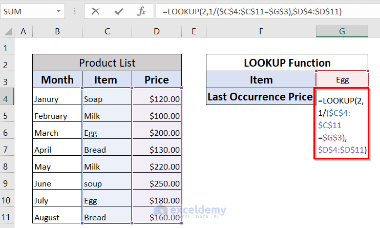
➤ We have to type the following formula in cell G4, and press Enter.
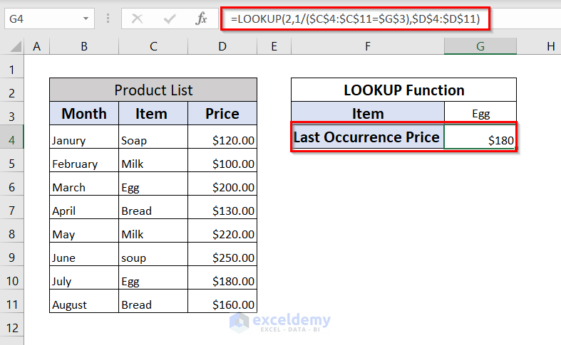
=LOOKUP(2,1/($C$4:$C$11=$G$3),$D$4:$D$11)This is how the formula works:
- The lookup value is 2 because the lookup function will find 2 through the column. When it reaches an error, it will return to its nearest value, 1, and show that result. The result will be $180.
- The lookup range is 1/($C$4:$C$11=$G$3) – returns 1 if it finds any match and an error if no match is found. The lookup value Egg, the array would be {#DIV/0!;#DIV/0!;1;#DIV/0!;#DIV/0!;#DIV/0!;1#DIV/0!}.
- The third parameter, $D$4:$D$11, is the range from which it’ll return the result, which are prices here.
➤ We can see the Last Occurrence Price of Egg is $180, the formula in the Formula Bar.
Method 3 – Using INDEX and MATCH Functions
Determine the Last Occurrence Price of the Egg using the INDEX and MATCH functions.
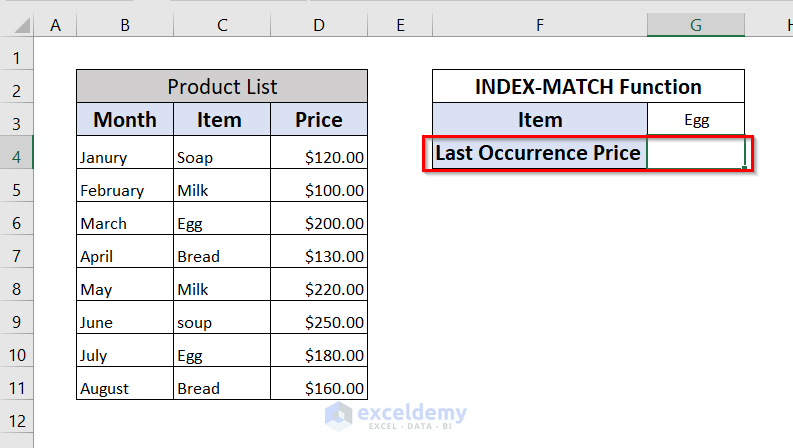
➤ Type the following formula in cell G4.
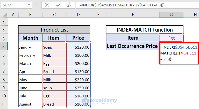
=INDEX($D$4:$D$11,MATCH(2,1/(C4:C11=G3)))In the formula,
- $D$4:$D$11 is the column range that contains the value we will return
- C4:C11 is the column range we are looking for
- G4 contains the criteria you will do the search based on.
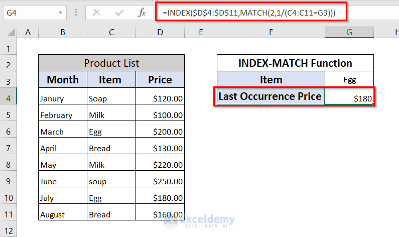
➤ Press Enter.
➤ See the Last Occurrence Price of Egg is $180.
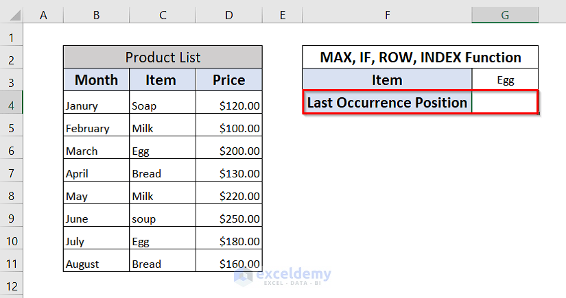
Method 4 – Combination of MAX, IF, ROW, and INDEX Functions
Find the Last Occurrence Position of Egg in cell G4. We will use a combination of MAX, IF, ROW, and INDEX functions.
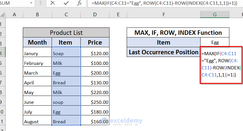
➤ Type the following formula in cell G4.
=MAX(IF(C4:C11="Egg", ROW(C4:C11)-ROW(INDEX(C4:C11,1,1))+1))In this formula,
=ROW(C3:C7)-ROW(INDEX(C4:C11,1,1))+1⟶ provides the relative position of the rows within the range C4:C11. You will find an array as a result.
=IF(C4:C11=”Egg”, ROW(C4:C11)-ROW(INDEX(C4:C11,1,1))+1)⟶ IF will check whether every value within the range C4:C11 is equal to “Egg”, returns the relative position when TRUE, returns FALSE.
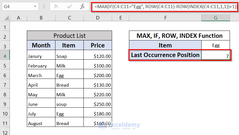
=MAX(IF(C4:C11=”Egg”, ROW(C4:C11)-ROW(INDEX(C4:C11,1,1))+1))⟶ the MAX function will test the array result we find from the IF function and provides the highest value from the resultant array. So, the last occurrence of text string “Egg” in range C4:C11 will be returned. It is 7.
➤ Press Enter.
➤ See the Last Occurrence Position of the Item Egg in cell G4.
Method 5 – Find Last Occurrence of a Value in a Column Using VBA Code
Use VBA code to find the last occurrence of a value in a column in Excel.
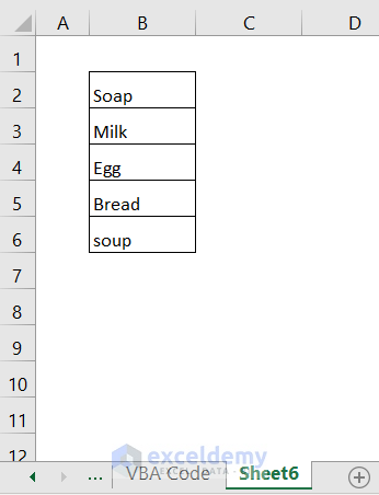
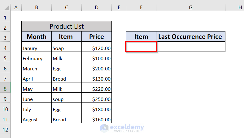
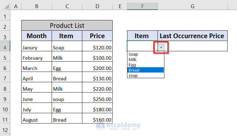
➤ Copy the unique items from the main sheet to a new sheet. Put the unique items in Sheet6.
➤ Go to the main sheet and click on any cell. Click on cell F4.
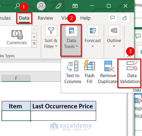
➤ Go to the Data tab in the Ribbon.
➤ Cick Data Tools.
➤ Select Data Validation.
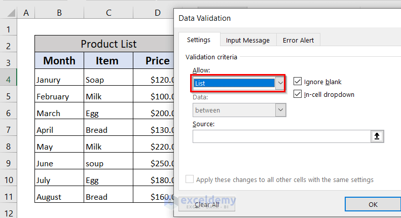
 ➤ A Data Validation window will appear.
➤ Select List from the Allow bar.
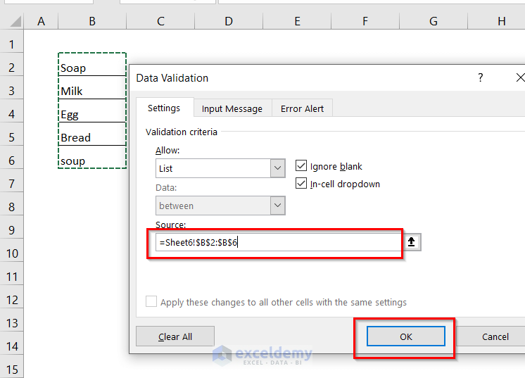
➤ Give a source in the Source box.
➤ Select the unique items from Sheet6 as our Source.
➤ Click OK.
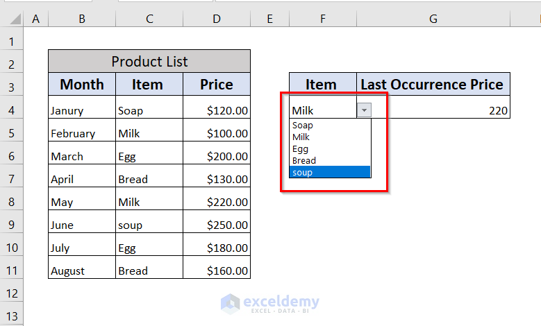
➤ We can see a down arrow sign is shown on the right side of our selected cell F4. Select any item name. Save our time because we won’t need to type the items every time.
➤ Make a new function named LastOccur with Excel VBA.
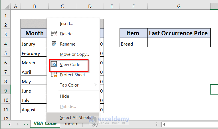
➤ We will right-click on our sheet name.
➤ We will select View Code from the context menu.
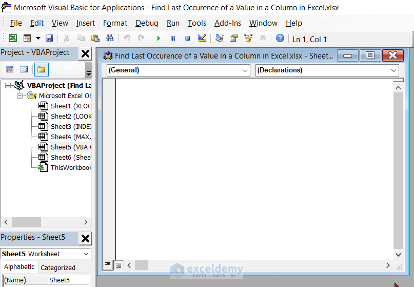
➤ A VBA window will appear.
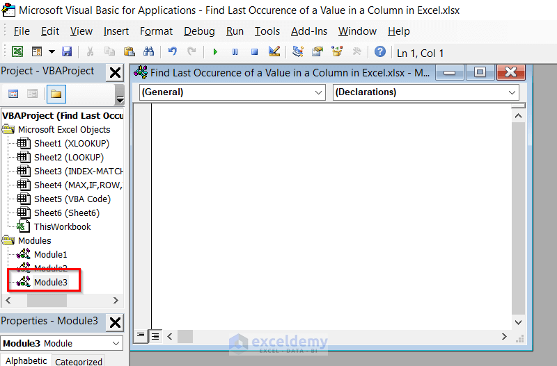
➤ Click on the Insert tab and select Module.
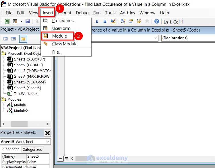
➤ Module 3 appears along with a window.
➤ Type the following code in that window.
Function LastOccur(LValue As String, LRange As Range, ColNum As Integer)

Dim l As Long

For l = LRange.Columns(1).Cells.Count To 1 Step -1

If LValue = LRange.Cells(l, 1) Then

LastOccur = LRange.Cells(l, ColNum)

Exit Function

End If

Next l

End Function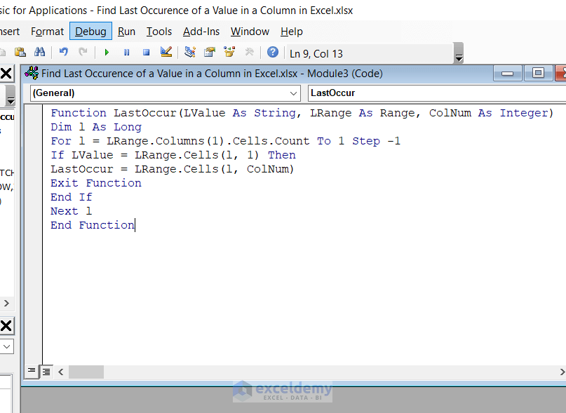
➤ Go to our active sheet and we will type the following formula in cell G4.
=lastOccur(F4,C4:D11,2)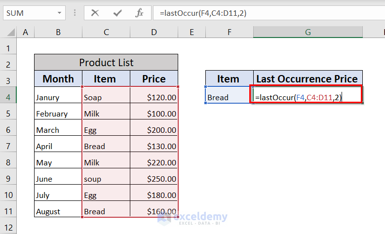
➤ The Last Occurrence Price of Bread in cell G4.
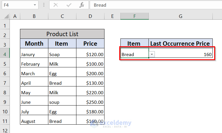
➤ See the last occurrence price of any item by clicking the down arrow situated right side of cell F4.
Download Workbook
Related Articles
- How to Find Last Non Blank Cell in Row in Excel
- How to Find Last Cell with Value in Column in Excel
- How to Find Last Cell with Value in a Row in Excel
- Find Last Value in Column Greater than Zero in Excel
<< Go Back To Excel Last Value in Range | Excel Find Value in Range | Excel Range | Learn Excel
Get FREE Advanced Excel Exercises with Solutions!

This VBA formula works like a charm for me. Thank you very much!
I could solve my issue with some array functions, but since my data set is over 60000 rows and 30+ columns, Excel isn’t happy with my array functions.
Instead, if I wanted to include some criteria e.g.,
if column C is 0, go to second last result, OR if column D is “text value”, go to second last result.
Hello, Niki!
Thanks for sharing your problem with us!
You can use the formula to find the second last result from a certain cell.
For this,
1. Select the cell where you want to see the result.
2. Insert the formula into the formula bar.
=INDEX(D:D,LARGE(IF(D:D<>"",ROW(D:D)),2))3. Press Shift + Ctrl + Enter.
Note: You have to press Shift + Ctrl + Enter together, otherwise the formula won’t work.
Can you please send me your dataset at ([email protected]), so that I can help you?
Hope this will help you!
Good Luck!
Regards,
Sabrina Ayon
Author, ExcelDemy.