Dataset Overview
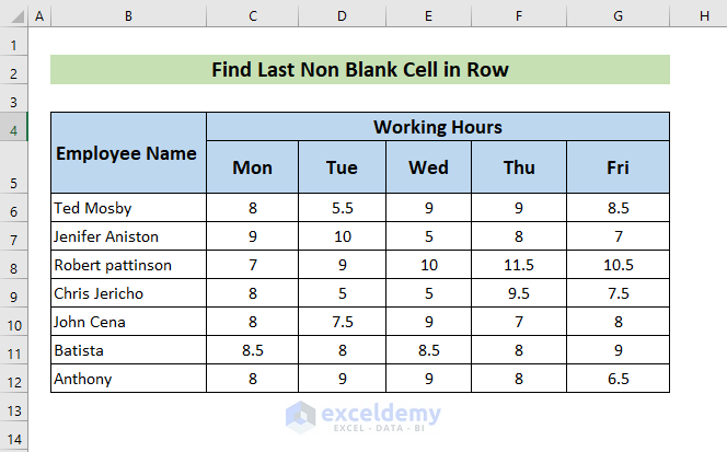
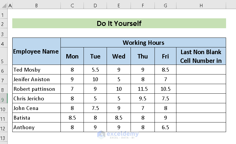
We’ll use the below Dataset containing Employee Names and Working Hours.
Method 1 – Using Excel LOOKUP Function
The LOOKUP Function is an easy way to find the last non- blank cell in row.
Steps:
- Select a cell (e.g., H6) where you want to apply the LOOKUP function.
- Enter the formula:
=LOOKUP(2,1/(B6:G6<>""),B6:G6)- The LOOKUP function searches through the range B6:G6 based on the lookup value (2) and returns the value of the last non-blank cell.
![]()
- Press ENTER.
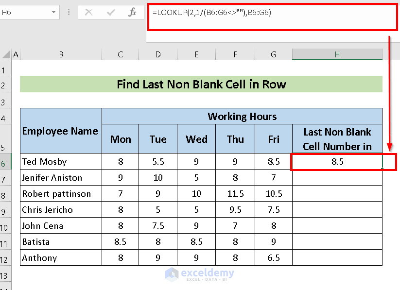
- Use the Fill Handle to Autofill the formula for other cells in the row
![]()
Method 2 – Combination of INDEX & COUNTA Functions
This method combines the INDEX and COUNTA functions.
Steps:
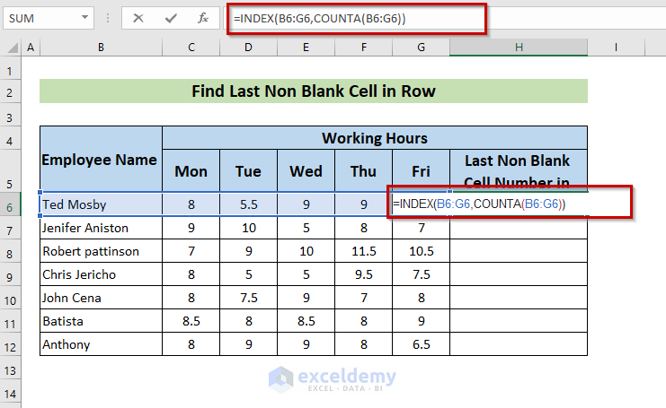
- Choose a cell (e.g., H6) where you want to apply the formula.
- Enter the formula:
=INDEX(B6:G6,COUNTA(B6:G6))- The COUNTA function counts the non-blank cell values in the range, and the INDEX function returns the value based on the range.
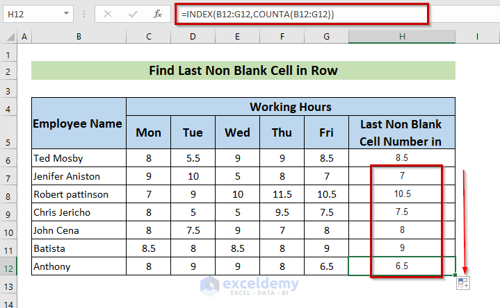
- Press ENTER.
![]()
- Use the Fill Handle to Autofill the formula for other cells in the row.
Method 3 – Using OFFSET Function
The OFFSET function is commonly used to find the last non-blank cell in a row.
Steps
- Select a cell (e.g., H6) to apply the method.
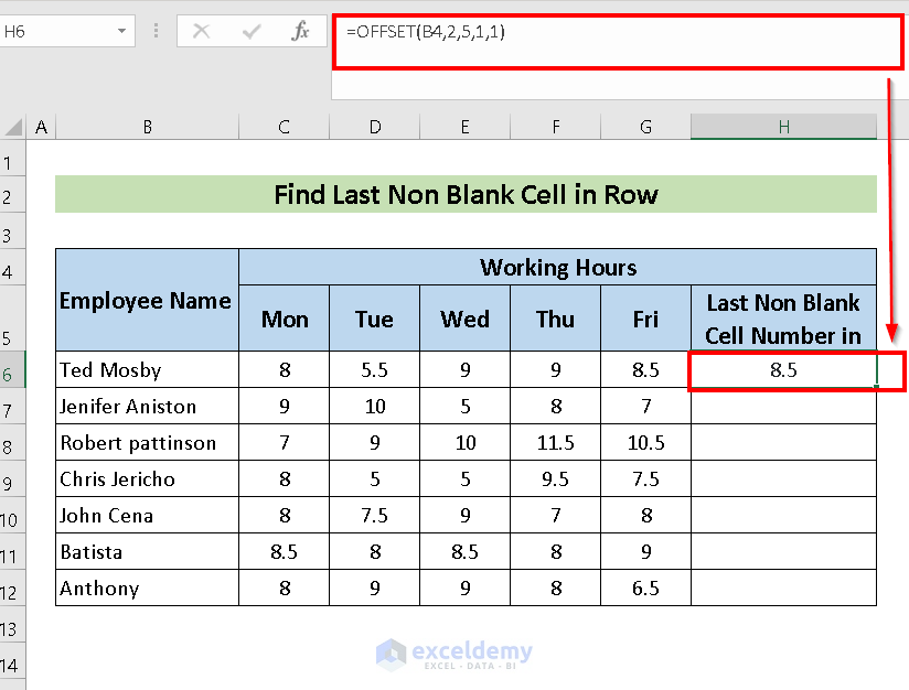
- Apply the formula:
=OFFSET(B4,2,5,1,1)Here,
- B4 is the starting point (reference cell).
- 2 represents the number of rows to ignore from the reference cell.
- 5 represents the number of columns to ignore to the right from the reference cell.
- 1 is the height (number of rows) of the output cell.
- 1 is the width (number of columns) of the output cell.
![]()
- Press ENTER.
- Autofill the formula for other cells in the row.
![]()
Method 4 – Using SUMPRODUCT Function
This method involves SUMPRODUCT along with INDIRECT, ROW, and MAX functions.
Steps
- Select a cell (e.g., H6).
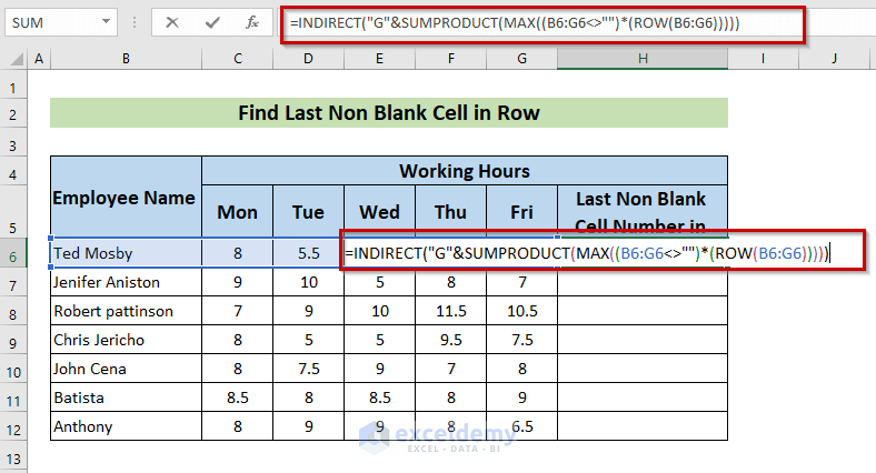
- Employ the formula:
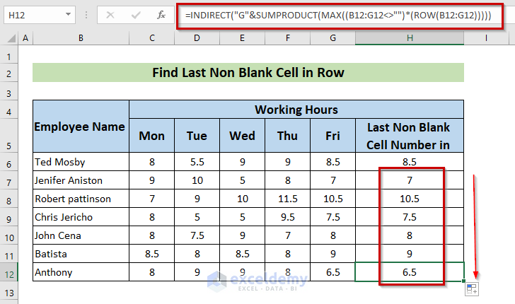
=INDIRECT("G"&SUMPRODUCT(MAX((B6:G6<>"")*(ROW(B6:G6)))))-
- Explanation:
- SUMPRODUCT finds the total number of non-blank cells in the selected range.
- INDEX function returns the value based on the location.
- INDIRECT function helps find the last non-blank cell in the row
- Explanation:
Formula Breakdown
-
- ROW(B6:G6):
- The ROW function returns the value of the row number for the range B6:G6.
- In this case, the output is 6 (since the formula is applied to row 6).
- MAX((B6:G6<>“”)*(ROW(B6:G6))):
- Here, we multiply the boolean result of (B6:G6<>””) with the row number from the previous step.
- The expression (B6:G6<>””) evaluates to an array of TRUE or FALSE values, where TRUE represents non-blank cells.
- Since all cells in this row are non-blank, the entire array is TRUE.
- Multiplying TRUE by the row number (6) results in an array of 6s.
- The MAX function then returns the largest value from this array, which is 6.
- SUMPRODUCT(MAX((B6:G6<>“”)*(ROW(B6:G6)))):
- The SUMPRODUCT function multiplies the maximum value (6) by 1 (since there’s only one value in the array).
- The result is still 6.
- INDIRECT(“G”&SUMPRODUCT(MAX((B6:G6<>“”)*(ROW(B6:G6))))):
- The INDIRECT function returns the value of a cell based on a text reference.
- We concatenate the letter “G” with the result from the previous step (6) using the ampersand (&).
- The final reference is “G6”.
- The INDIRECT function returns the value from cell G6, which is 8.5 in your dataset.
- ROW(B6:G6):
- Press ENTER.
![]()
- Autofill the formula for other cells in the row.
Method 5 – Applying XLOOKUP Function
The XLOOKUP function is an advanced function in Excel. We can use it here to find last non-blank cell in row.
Steps
- Choose a cell where you want to apply the formula. In this case, you’ve selected cell H6.
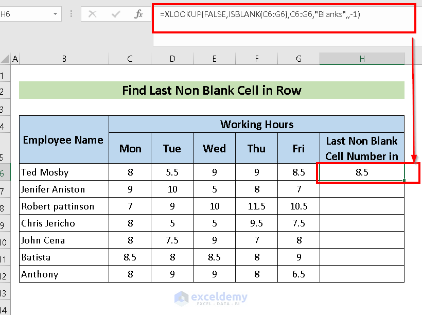
- Enter the following formula in cell H6:
=XLOOKUP(FALSE,ISBLANK(C6:G6),C6:G6,"Blanks",,-1)-
- The XLOOKUP function searches for a value (in this case, FALSE) within the specified array (C6:G6).
- The ISBLANK function checks if each cell in the array is blank and returns an array of TRUE or FALSE values.
- The C6:G6 range contains the values you want to search.
- The “Blanks” argument specifies the value to return if no match is found (in this case, it’s not relevant since we’re looking for non-blank cells).
- The empty argument (“”) is used to skip specifying a lookup value.
- The -1 argument indicates that the search should be from last to first (finding the last non-blank cell).
![]()
- After entering the formula, press ENTER to calculate the result.
- Use the Fill Handle (the small square at the bottom-right corner of the cell) to autofill the formula for other cells in the row.
![]()
Practice Section
For further practice, you can continue working with the methods mentioned above, using the information below:
Download Practice Workbook
You can download the practice workbook from here:
Related Articles
- How to Find Last Cell with Value in Column in Excel
- How to Find Last Cell with Value in a Row in Excel
- Find Last Value in Column Greater than Zero in Excel
- How to Find Last Occurrence of a Value in a Column in Excel
<< Go Back To Excel Last Value in Range | Excel Find Value in Range | Excel Range | Learn Excel
Get FREE Advanced Excel Exercises with Solutions!

Hi, how do you find the second last non blank value?
Sorry DIEGO for my late response.
There needs to make some changes in the formula in case of finding the second last non blank cell.
I have used the following formula using LOOKUP function in cells D5 to D15 that is the chemistry marks in the dataset to find the second last non-blank cell.
=LOOKUP(2,1/((D5:D15<>D15)*(D5:D15<>“”)),D5:D15)
My dataset is given below:
Second Last Non Blank Value
Name Physics Chemistry
Green 164 110 (D5)
Jack 185 165
Joey 178 132
Mark 183 137
Austin 165 112
Marvin 173 119
Mason 186 170
Mount 170
Martin 177 160
Freeman 164
Federer 163 111 (D15)
Second Last Non Blank Value 160
For me it worked perfectly. I hope it will work the same way for you too.
Hi, Thank you so much worked perfectly! Can you explain the vlookup arguments. Why is the first argument a “2”?
Hello MARIA, thanks for the comment and sorry for my late reply.
In the LOOKUP function, the first argument is Lookup_value. I have typed 2 just to signify the NUMBER format. You can type any number. It will work just fine.