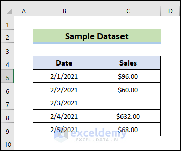
We have a simple dataset where we’ll find the last cell with a value in a column.
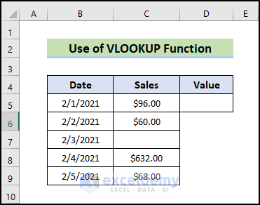
Method 1 – Inserting the LOOKUP Function to Find Last Cell with Value in Column in Excel
Case 1.1 – Using the Basic LOOKUP Function Only
We will check the column C.
Steps:
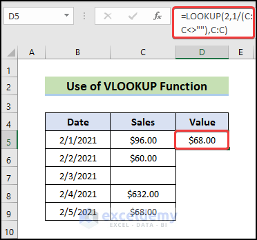
- Go to Cell D5.
- Insert the following formula:
=LOOKUP(2,1/(C:C<>""),C:C)- Hit Enter.
- We get the last value of Column C.
Note:
- C:C<>”” – Checks the whole Column C for empty cells and returns TRUE/FALSE for each cell of that range.
- 1/ – 1 will be divided with the value from the previous step, which may be TRUE or FALSE. For FALSE (i.e. a nonblank cell), the formula returns an error, #DIV/0! because we can’t divide any number by zero.
- 2 – The LOOKUP function attempts to locate 2 in the list of values produced in the last step. Since it can’t locate the number 2, it looks for the next maximum value, which is 1. It searches this value starting from the end of the list and proceeding to the start of this list. The process will end when it gets the first result. This will be the last cell in the range that contains a value.
- C:C – This is the last statement of the LOOKUP function, which is the range of cells that the function will fetch the corresponding value from.
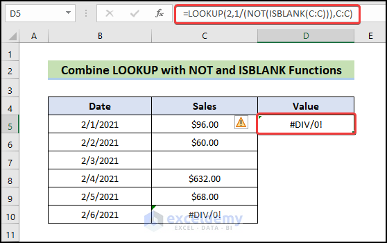
Case 1.2 – Combining LOOKUP, NOT, and ISBLANK Functions to Find the Last Cell with a Value in Column
Steps:
- In the 10th row, we added an error by dividing a number by 0.
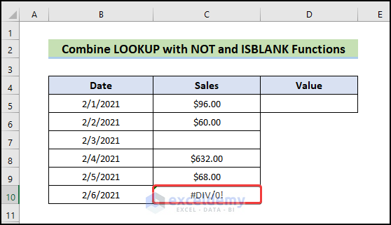
- Add the NOT and ISBLANK functions in the formula. The formula becomes:
=LOOKUP(2,1/(NOT(ISBLANK(C:C))),C:C)- Hit Enter.
- We can see that in the result section, an error value is showing. Usually, the LOOKUP function avoids this error value.
Case 1.3 – Applying LOOKUP and ISNUMBER Functions to Find the Last Cell with a Numeric Value in a Column
Steps:
- Add textual data in the 10th row.
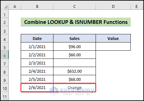
- Modify the original formula and add ISNUMBER so it becomes:
=LOOKUP(2,1/(ISNUMBER(C:C)),C:C)- Press Enter to get a return value.

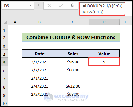
Case 1.4 – Using LOOKUP with the ROW Function to Find the Row Where the Last Value Exists
Steps:
- Modify the formula to the following:
=LOOKUP(2,1/((C:C)),ROW(C:C))- Hit Enter.
Read More: How to Find Last Row with a Specific Value in Excel
Method 2 – Finding the Last Cell with a Numeric Value in a Column Using Excel INDEX and COUNT Functions
Steps:
- Remove the blank cell and add textual values in the range. Add a blank cell as the last.
- Insert the following formula in the result cell:
=INDEX(C5:C10,COUNT(C5:C10))- Hit Enter.
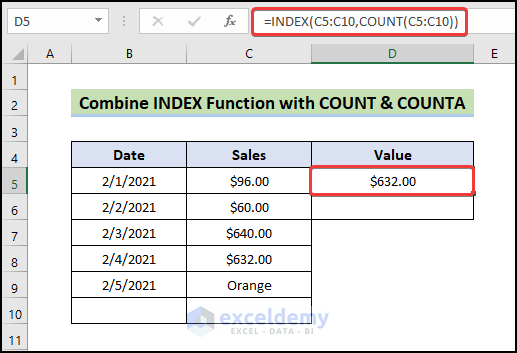
- We get only numeric values as we used the COUNT function.
- To get any results, use the following:
=INDEX(C5:C10,COUNTA(C5:C10))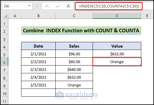
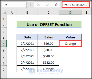
Method 3 – Applying the OFFSET Function to Find the Last Cell with a Value in a Column in Excel
Case 3.1 – Using the Basic OFFSET Function
Steps:
- Make sure there are no empty cells in the dataset.
- Write OFFSET and select Cell C5 as reference. The next two arguments are the number of rows and columns, respectively:
=OFFSET(C5,4,0)- Hit Enter.
Case 3.2 – Using the OFFSET and COUNT Functions to Find the Last Cell with a Value in a Column
Steps:
- Go to Cell D5.
- Insert the following function.
=OFFSET(C5,COUNT(C5:C10)-1,0)- Hit Enter.
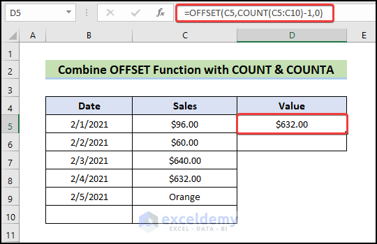
- To get any values (not just numeric ones), use the following formula:
=OFFSET(C5,COUNTA(C5:C10)-1,0)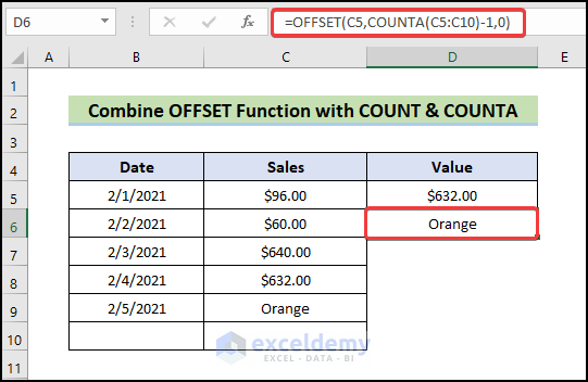
This formula doesn’t work if there are blank values inside the dataset.
Read More: How to Find Last Cell with Value in a Row in Excel
Download the Practice Workbook
Related Links
- How to Find Last Non Blank Cell in Row in Excel
- How to Find Last Cell with Value in a Row in Excel
- Find Last Value in Column Greater than Zero in Excel
- How to Find Last Occurrence of a Value in a Column in Excel
<< Go Back To Excel Last Value in Range | Excel Find Value in Range | Excel Range | Learn Excel
Get FREE Advanced Excel Exercises with Solutions!

Thanks for the info, will be following up with structured lessons
You are welcome, Ruben! Please share your thoughts with us, too. Regards.
Excellent. Useful formulas. Well explained in a very easy way.
Hello, Mubashir!
Thanks for your appreciation. To get more helpful content stay in touch with ExcelDemy.
Regards
ExcelDemy
Thank You!
I’ve been looking for a solution to referencing the last non empty cell in a sheet to another cell within the same sheet.
Took me a while and a lot of searching to find your solution.
But, it works great!
Thanks again!
Hello Abdrman,
You are most welcome.
Regards
ExcelDemy
I am using your solution 1.4 Using LOOKUP with ROW Function to Find Row Where Last Value Exists. I tried to modify it to lookup the information on another sheet, but it is returning #NAME? instead of the row number.
I am using this: =LOOKUP(2,1/((Week_1!B:Week_1!B)),ROW(Week_1!B:Week_1!B))
Hello JULI
Thanks for visiting our blog and sharing your query. You can modify the formula mentioned in example 1.4 and find the last cell with a number value on another sheet:
=LOOKUP(2,1/(Week_1!C:C),ROW(Week_1!C:C))I hope the formula will overcome your issue; good luck.
Regards
Lutfor Rahman Shimanto
ExcelDemy
I’d like to use the same formula throughout my spreadsheet. I have a column for dollars BA40:BA61, I want to know the last number. BA40:BA50 are blank, BA51:BA55 have dollars, BA56:BA61 do not yet have data. If I use the formula =INDEX(BA50:BA61,COUNT(BA50:BA61)) it yields the 2nd last number. If I expand the range to say BA40:BA61 it yields blank. Only if I correct the formula to start at the first instance of data B51 does it give the proper value =INDEX(BA51:BA61,COUNT(BA51:BA61)). This forces me to manually change my formulas to suit the data. If I use the CountA function, no joy.
Please help.
Hello Dave Woodward,
You can use the following formula to always get the last number in your range, even if there are blanks at the beginning or end.
Formula:
=LOOKUP(2,1/(BA40:BA61<>“”),BA40:BA61)
This formula works by looking for the last non-blank value in the entire range BA40:BA61, so you don’t have to change it even if your data shifts. It ignores blanks at the start, end, or in the middle.
Regards
ExcelDemy