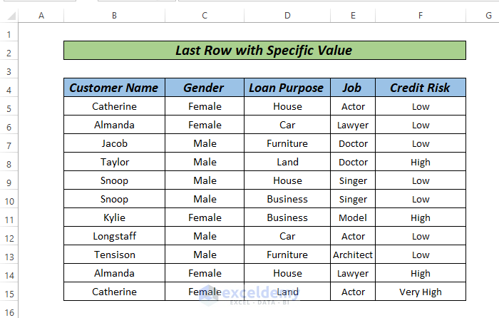
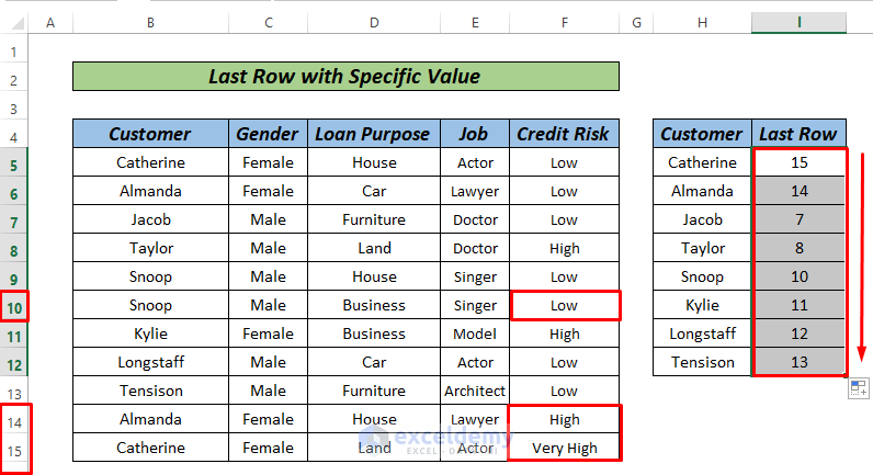
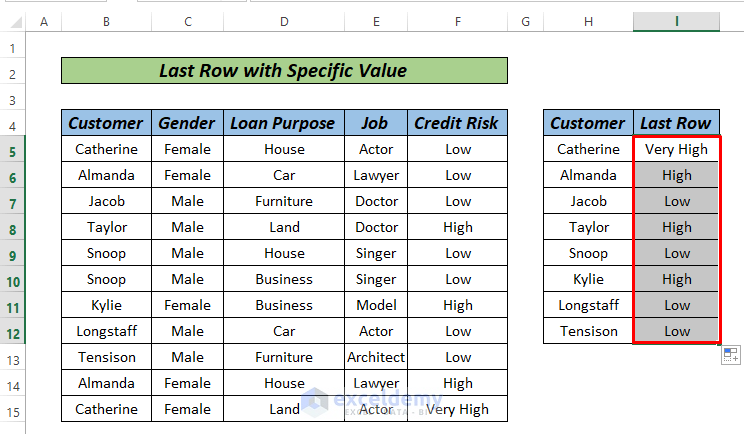
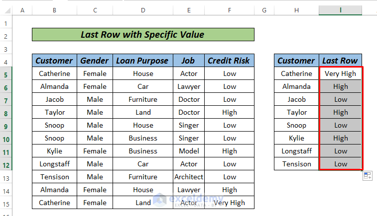
Here, we have a sample dataset containing Customer Name, Gender, Loan Purpose, Job, and Credit Risk. The dataset is repetitive. Snoop, Almanda, and Catherine have data more than once. We want to know their last Credit Risk data.
Method 1 – Finding the Last Row with a Specific Value Using the MAX Function
Steps:
- Enter the following Formula in cell I5:
=MAX(IF($B$5:$B$15=H5,ROW($B$5:$B$15)))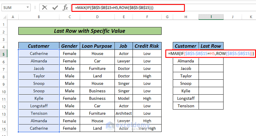
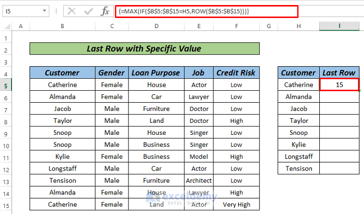
- Press the CTRL+SHIFT+ ENTER key. ( If you are using Excel’s updated version from 2019, only pressing ENTER key will do).
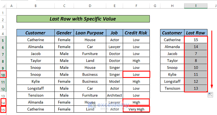
- Drag down to AutoFill rest of the series.
Formula Breakdown
- IF($B$5:$B$15=H5,ROW($B$5:$B$15)) yields the result as {5;FALSE;FALSE;FALSE;FALSE;FALSE;FALSE;FALSE;FALSE;FALSE;15}. Where 5 and 15 indicate the Row number for Catherine.
- The MAX Function will take 15 as the maximum number and give us the result.
- Explanation: This array formula checks each cell in column A for “Value“. If true, it multiplies the row number by 1, otherwise by 0. MAX returns the highest row number where “Value” is found.
- Benefits: This method is simple and straightforward. You can use it for small to medium datasets where array formulas are manageable.
Read More: How to Use Excel Formula to Find Last Row Number with Data
Method 2 – Using the SUMPRODUCT Function to Find the Last Row with a Specific Value
Steps:
- Enter the following formula in cell I5:
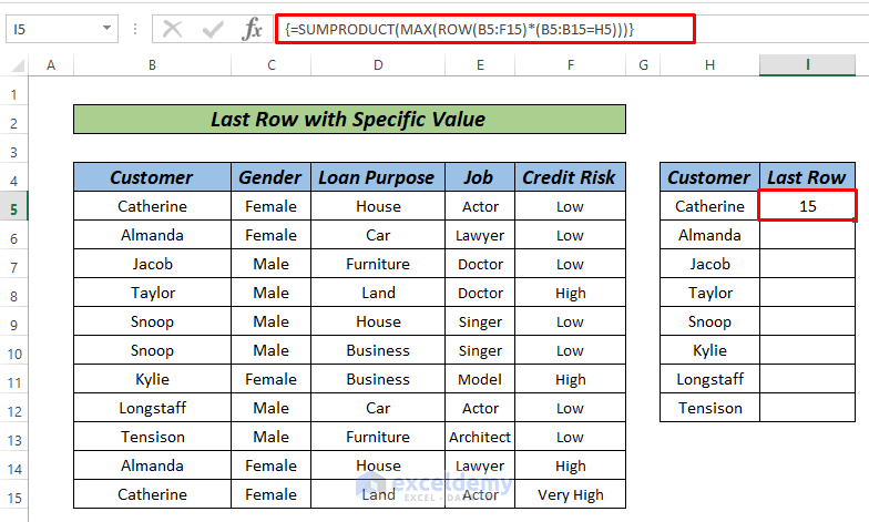
=SUMPRODUCT(MAX(ROW(B5:F15)*(B5:B15=H5)))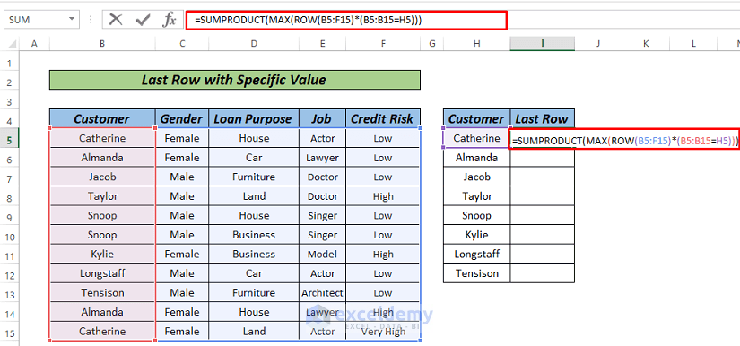
- Press ENTER or CTRL+SHIFT+ENTER
- Drag down to AutoFill rest of the series.
Formula Breakdown
- ROW(B5:F15)*(B5:B15=H5) gives us the output as {5;0;0;0;0;0;0;0;0;0;15}
- SUMPRODUCT(MAX{5;0;0;0;0;0;0;0;0;0;15}) will give the final output as 15.
- Explanation: It is similar to the MAX function but uses SUMPRODUCT to handle the array, returning the maximum row number where “Value” is found.
- Benefits: You can avoid array formulas, which can be complex. You can use this formula if you prefer non-array formulas for better readability and maintenance.
Method 3 – Finding the Last Row with a Specific Value by the INDEX Function
Steps:
- Enter the following formula in cell I5:
=INDEX($F$5:$F$15,SUMPRODUCT(MAX(ROW($B$5:$B$15)*(H5=$B$5:$B$15))-4))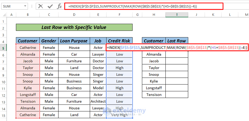
- Press ENTER.
- Drag down to AutoFill rest of the series.
Here, the function SUMPRODUCT(MAX(ROW($B$5:$B$15)*(H5=$B$5:$B$15))-4 gives us the result 11. 11 indicates the Row number in the table. As you can see, the last row in the worksheet is 15, but the data in our table started from Row 5, so we use -4 in the formula.
Then, the formula =INDEX($F$5:$F$15,11) will return a Very High output.
Explanation: It works by identifying the row numbers in B5 where the value matches H5, calculating the maximum row number from these matches, adjusting it for the starting row, and then using INDEX to return the corresponding value from F5.
Benefits: This method is dynamic, avoids array formulas, and is versatile for finding the last occurrence of a value in one column and retrieving a related value from another column.
Method 4 – Finding the Last Row with a Specific Value in Excel Using the LOOKUP Function
Steps:
- Enter the following formula in cell I5:
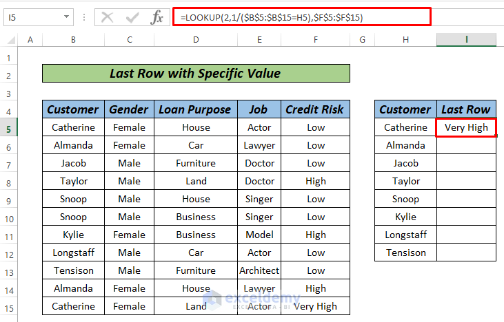
=LOOKUP(2,1/($B$5:$B$15=H5),$F$5:$F$15)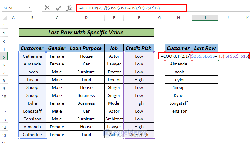
- Press ENTER.
- Drag down to AutoFill rest of the series.
- LOOKUP searches for the last occurrence of “Value” in column A and returns the corresponding row number. The LOOKUP function then searches for the value 2 (which will never be found) but, due to its lookup behavior, returns the last numerical match (i.e., the last 1) and uses that position to fetch the corresponding value from F5.
- Explanation: This formula finds the last occurrence of a specific value (H5) in the range B5 and returns the corresponding value from F5. It does this by creating an array where each element is 1 if the corresponding element in B5 equals H5 and #DIV/0! otherwise.
- Benefits: This method is efficient and easy to implement for locating the last match in a dataset.
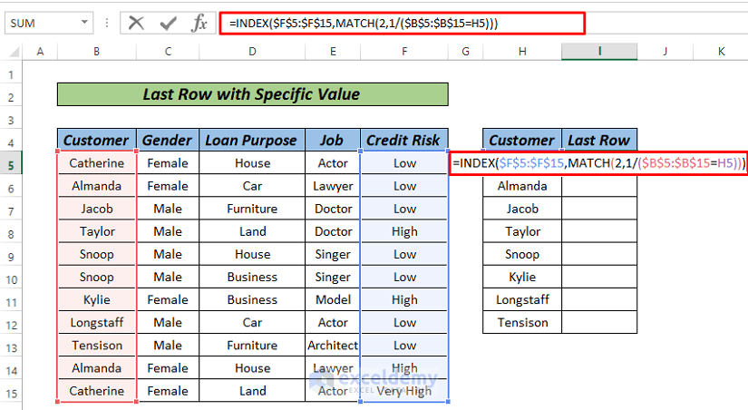
Method 5 – Finding the Last Row with a Specific Value by the MATCH Function
Steps:
- Enter the following formula in cell I5:
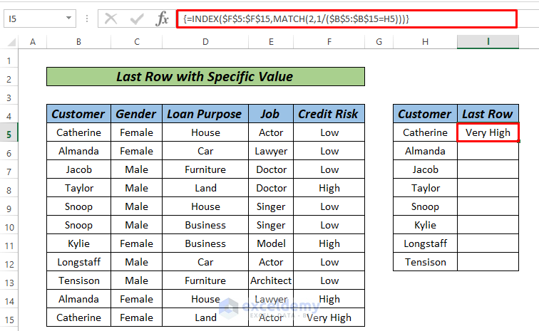
=INDEX($F$5:$F$15, MATCH(2, 1/($B$5:$B$15=H5)))
- Explanation: This formula finds the last row with a specific value (H5) in the range B5 and returns the corresponding value from F5. It uses MATCH to locate the last occurrence of H5 by creating an array of 1s and #DIV/0! errors, where 1 corresponds to matches. MATCH searches for 2, which ensures it returns the position of the last 1. INDEX then uses this position to fetch the value from F5.
- Benefits: Compatible with dynamic arrays. You can use it for dynamic tables and newer Excel versions.
- Press ENTER or CTRL+SHIFT+ENTER
- Drag down to AutoFill the rest of the series.
Method 6 – Finding the Last Row with a Specific Value by VBA
Steps:
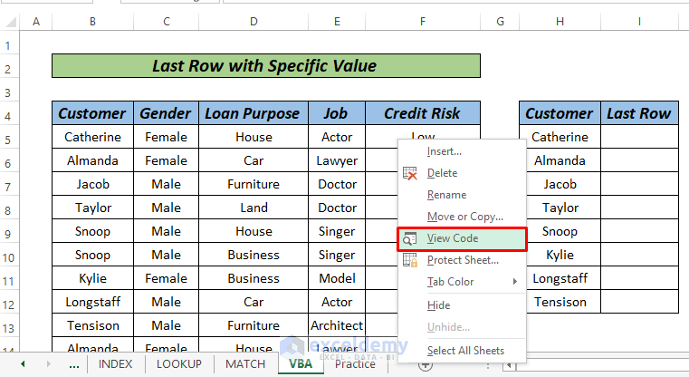
- Right-click on the sheet and go to View Code.
- Enter the VBA code below.
VBA Code:
Option Explicit
Function MylastrowFunction(SpecificValue As String, SpecificRange As Range, LastColumnNumber As Integer)
Dim i As Long
For i = SpecificRange.Columns(1).Cells.Count To 1 Step -1
If SpecificValue = SpecificRange.Cells(i, 1) Then
MylastrowFunction = SpecificRange.Cells(i, LastColumnNumber)
Exit Function
End If
Next i
End Function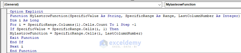
- Press F5 or the play button to run the code.
- Enter the following formula in cell I5:
=MylastrowFunction(H5,B5:F15,5)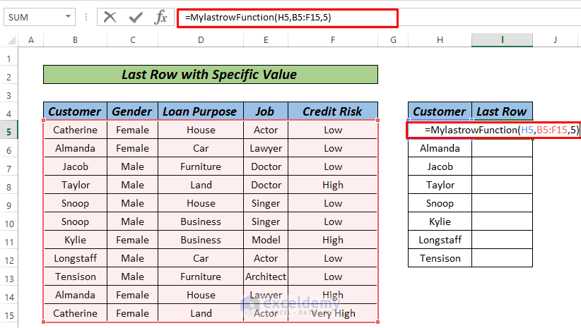
- Explanation: This user-defined VBA function loops through each cell in the specified range and checks if it matches the value. It updates the variable to the current row number when a match is found.
- Finds the last occurrence of SpecificValue in SpecificRange and returns the value from the specified column (LastColumnNumber).
- Iterates from the last row to the first row in SpecificRange.
- Check if the cell in the first column matches SpecificValue.
- Returns the value from the LastColumnNumber of the matching row and exits the function.
- Benefits: It’s an automated solution. Useful for repetitive tasks or when you want to create a reusable function.
- Press ENTER or CTRL+SHIFT+ENTER.
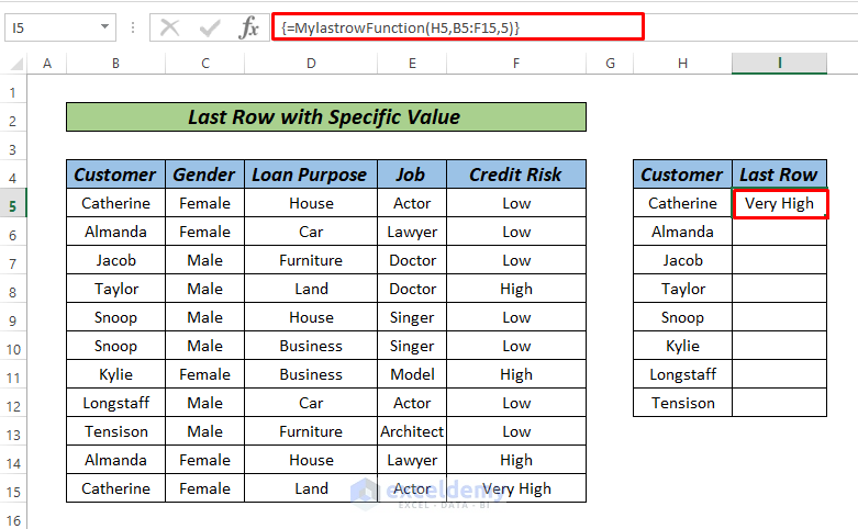
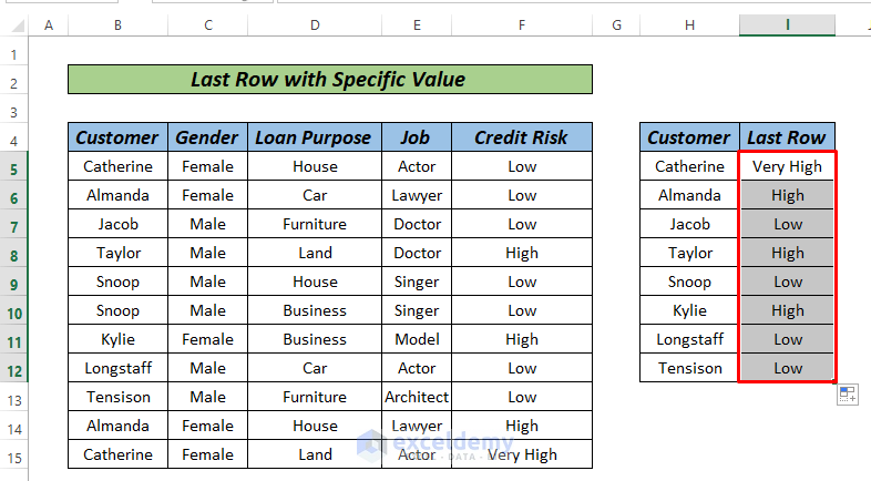
- Drag down to AutoFill the rest of the series.
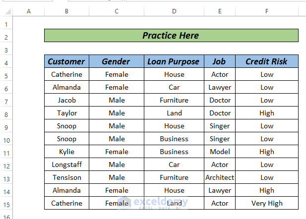
Practice Section
We’ve attached a practice workbook where you may practice these methods.
Download the Practice Workbook
Related Articles
- How to Find Last Non Blank Cell in Row in Excel
- How to Find Last Cell with Value in Column in Excel
- Excel Find Last Column With Data
- How to Find Highest Value in Excel Column
- How to Find Lowest Value in an Excel Column
- How to Find Last Cell with Value in a Row in Excel
<< Go Back to Find Value in Range | Excel Range | Learn Excel
Get FREE Advanced Excel Exercises with Solutions!

Please can this be updated to explain how each example works? It’s hard to generalize from these single examples to understand how to adapt the formulae for my own spreadsheets.
Give a man a fish and you feed him for a day; teach him to fish and you feed him for a lifetime. Thanks for the 5 fish 🙂
Hello Anonymous,
Thank you for your feedback! I’ve updated the document to include detailed explanations for each example, showing exactly how each formula works step-by-step. This should make it easier for you to understand how to adapt the formulas for your own spreadsheets.
I’m glad the initial examples were helpful, and I hope the added explanations will provide the deeper understanding you’re looking for. If you have any more questions or need further clarification, please feel free to ask. Happy spreadsheeting!
Regards
ExcelDemy