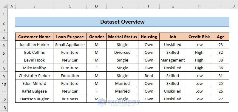
Consider the following dataset about different customers who have applied for a bank loan. We will find the last cell with data in a row.
Method 1 – Using a Keyboard Shortcut to Find the Last Cell with Value in a Row in Excel
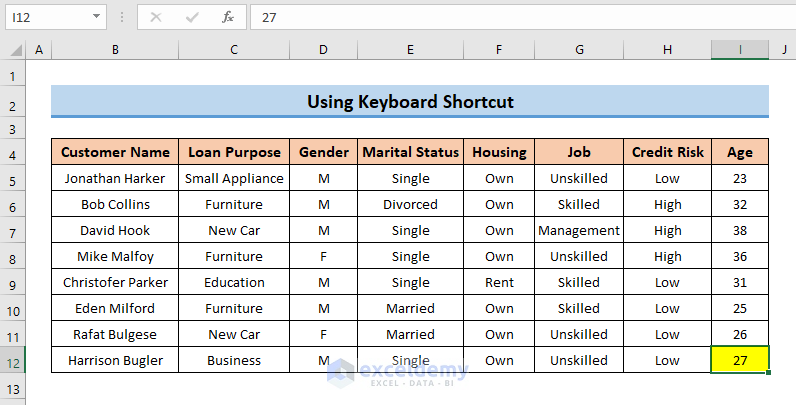
- Click on the row’s first cell and press Ctrl + Right Arrow.
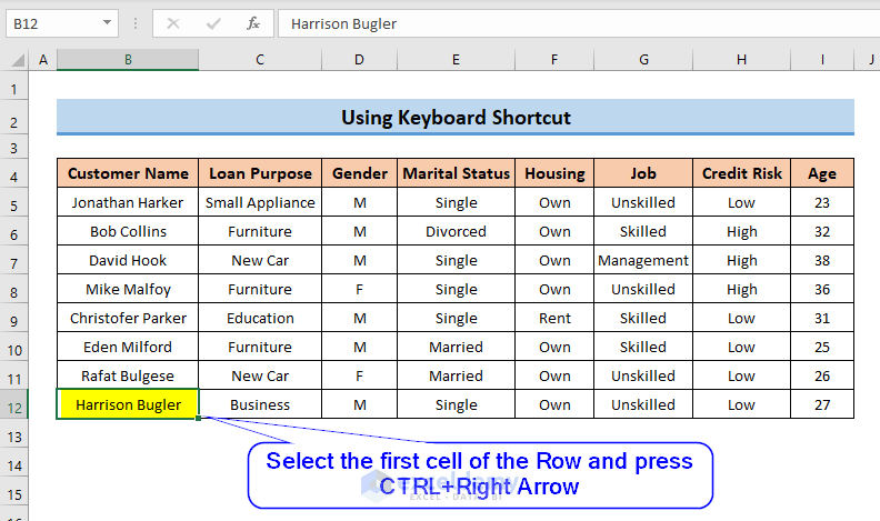
- Your cursor will move to the last non-empty cell in that row.
Read more: How to Find Last Cell with Value in Column in Excel
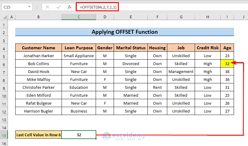
Method 2 – Getting the Last Cell with Value in a Row with the OFFSET Function in Excel
If you know the number of columns and rows of your dataset, you can find the last cell value in any row by using the OFFSET function.
- To find out the last cell value in Row 6, type the formula in an empty cell,
=OFFSET(B4,2,7,1,1)- B4 = First cell of the dataset
- 2 = Number of the row of your dataset excluding the first row
- 7 = Number of the column of your dataset excluding the first column
- 1 = cell height
- 1 = cell width
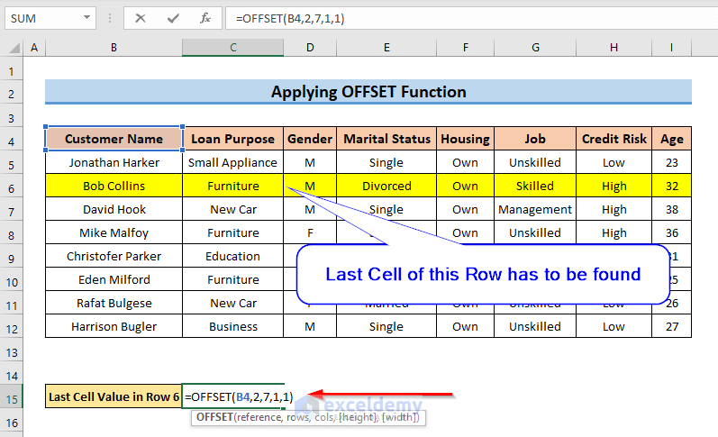
- Press Enter and you will find the value of the last cell of Row 6.
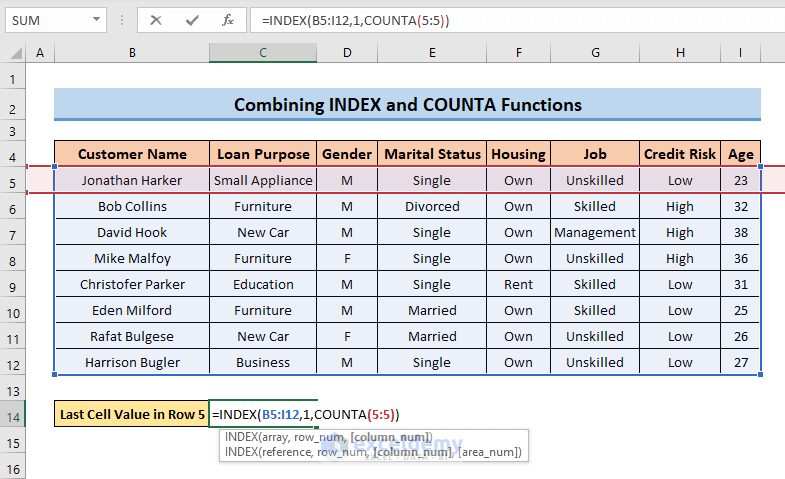
Method 3 – Using Excel INDEX and COUNTA Functions to Find the Last Non-Blank Cell in a Row
- To find the last cell value in Row 5, use the following formula in an empty cell,
=INDEX(B5:I12,1,COUNTA(5:5))- 5:5 = Row 5
- B5:I12 = Array
- 1 = row_num
- Here’s the result.
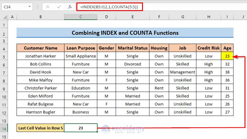
Formula Breakdown
↪️ The COUNTA function counts the number of cells in a range that are non-empty.
COUNTA(5:5) returns the total number of non-empty cells in Row 5 => 8
↪️ INDEX(B5:I12,1,COUNTA(5:5)) = INDEX(B5:I12,1,8) = 23
Output => 23
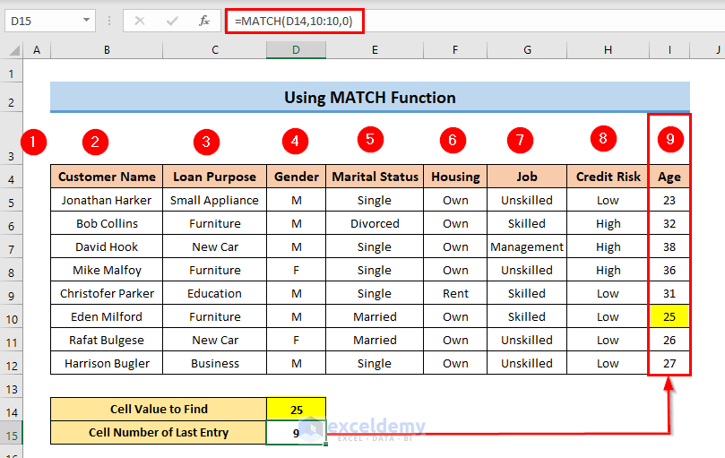
Method 4 – Using the MATCH Function to Find the Last Cell with Value in a Row in Excel
- We know the value that we’re searching for in row 10 and want to find the column number relative to the start of the dataset.
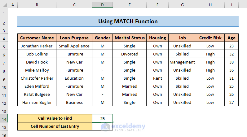
- Use the following formula:
=MATCH(D14,10:10,0)- D14 = lookup_value
- 10:10 = Row 10
- 0 = Exact match
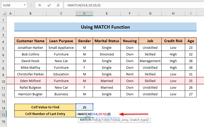
- You will find the number of the last non-empty cell of Row 10.
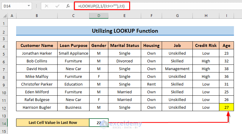
Method 5 – Finding the Last Cell Value in a Row Using the Excel LOOKUP Function
- Use the following formula:
=LOOKUP(2,1/(I:I<>""),I:I)I:I = Last column of the dataset
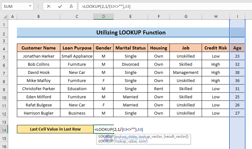
- You will find the value of the last cell of the last row of the dataset.
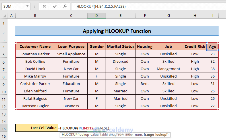
Method 6 – Applying the HLOOKUP Function to Find the Last Cell with Value in a Row in Excel
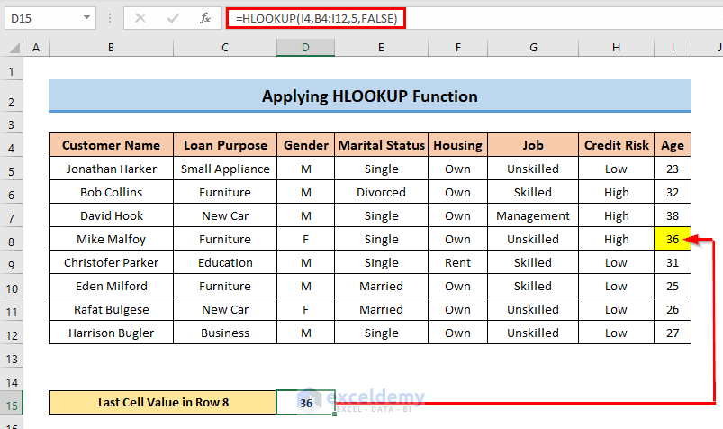
We will find the last cell of Row 8 in our dataset.
- Use this formula in an empty cell,
=HLOOKUP(I4,B4:I12,5,FALSE)- I4= Last column of the first row (Reference cell)
- B4:I12 = Range of Dataset
- 5 = 5th Row of our dataset including the reference cell’s row
- FALSE = Exact Match
- You will find the value of the last cell of Row 8.
Read More: How to Find Last Non Blank Cell in Row in Excel
Download the Practice Workbook
Further Readings
- How to Find Last Non Blank Cell in Row in Excel
- How to Find Last Cell with Value in Column in Excel
- Find Last Value in Column Greater than Zero in Excel
- How to Find Last Occurrence of a Value in a Column in Excel
<< Go Back To Excel Last Value in Range | Excel Find Value in Range | Excel Range | Learn Excel
Get FREE Advanced Excel Exercises with Solutions!

How do you do #3 above, but pulling from another workbook? Thank you!
Hello ANTHONY,
Here, we’ll get the value of the last cell of a row and show it in cell C14.
But, as per your condition, we’ll retrieve this value from another workbook named Sales. Now, we want to extract the value of the last cell of Row 5 from the Dataset worksheet of this workbook.
To do this,
• At first, select cell C14 and call the INDEX function.
• Then, select cells in the B5:E5 range.
• After that, insert the COUNTA function and select the same range as the argument.
• As usual, press the ENTER button.
• Finally, you can see the result in cell C14 and the final form of the formula is like the following.
=INDEX([Sales.xlsx]Dataset!$A$5:$D$5,COUNTA([Sales.xlsx]Dataset!$A$5:$D$5))Here, the part inside the square brackets are the name of the workbook. And the part before the exclamation mark and after the square bracket is the name of the worksheet.
That’s how you can do it from another workbook. It’s all from me on this topic. Follow our website, ExcelDemy, a one-stop Excel solution provider, to explore more.
Awesome, thank you that was helpful! Any chance you know how to reference 2nd to last cell with data from the other workbook?
Hello ANTHONY,
If your second to the last row is situated in Row 11, then you can use the following formula.
=INDEX(‘[Sales.xlsx]Dataset’!$A$11:$H$11,COUNTA(‘[Sales.xlsx]Dataset’!$A$11:$H$11))
You have to just change the reference according to the position of your desired row.
Best Regards
Tanjima Hossain
Hi, how you can exclude a specific value thorugh the whole row?
Hello PEDRO,
As per your question, I will try to show an easier way to remove a specific value from a row. Here, we have the specific text “Furniture” in three rows which we will remove from these rows.
• Go to the Home tab >> Find & Select dropdown >> Replace option.
Then, you will have the Find and Replace dialog box.
• Type Furniture in the Find what box, and blank in the Replace with box.
• Click on Replace All.
Then, a message box will notify you about the number of replacements.
In this way, we have removed Furniture from three rows.
If you want to remove this specific text from a specific row only, then before doing the stated procedures just select that specific row.
Best Regards,
Tanjima Hossain