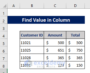
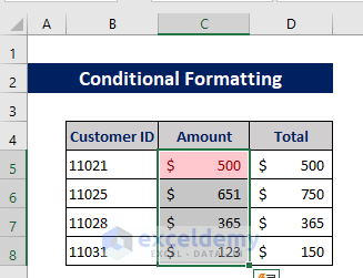
Let’s take a dataset of some customers in a Super shop with the Customer ID, shopping Amount on a particular date, and also a Total if they bought anything previously. We’ll use it to demonstrate how you can find values in a column.
How to Find Value in Column in Excel: 4 Methods
Method 1 – Apply Conditional Formatting Feature to Find Value in a Column in Excel
Here we will find a particular value in an Excel spreadsheet.
Steps:
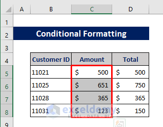
- Select the column where we want to find the value. We selected Cells C5 to C8 in Column C.
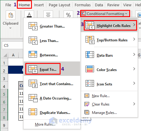
- Go to the Home tab.
- Select the Conditional Formatting.
- Choose Highlight Cells Rules from the drop-down for Conditional Formatting.
- Select Equal To.
- You will get a Pop-Up.
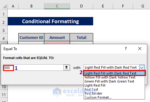
- We want to find a value which is 500, so put this value on the first section on the following image.
- You can also choose the highlight color. Select it from the menu as in the following image.
- You will find the value colored on the selected column.
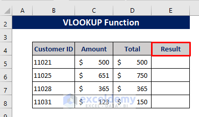
Method 2 – Using Excel VLOOKUP Function to Find Value in a Column
Steps:
- Create a new column named Result to show the VLOOKUP.
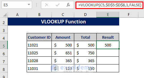
- Go to Cell E5 and type the VLOOKUP function. Here we will find the Cell D5 from the column range D5 to D8. We put FALSE in the argument section because we need the exact result.
- So, the formula becomes:
=VLOOKUP(C5, D5:D8,1,FALSE)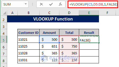
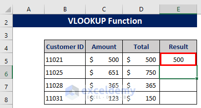
- Press Enter. As our selected value is found on the selected column, we will see that on this cell.
We can also compare all the values of Column D with Column E. Some additional steps are needed for that:
- Edit the formula to put dollar ($) sign to use Absolute Reference:
=VLOOKUP(C5,$D$5:$D$8,1,FALSE)- Press Enter.
- Pull down the Fill Handle icon from Cell E5.
- Get the result of comparing Column D values on Column C.
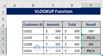
Here we see that the values from cells D5 and D7 are found in Column C. And the rest of the values do not exist in Column C. So, the function will return #N/A errors for them.
Note: In the case of VLOOKUP, the comparing column must be on the right side of the reference cell. Otherwise, this function will not work.
Read More: How to Find Multiple Values in Excel
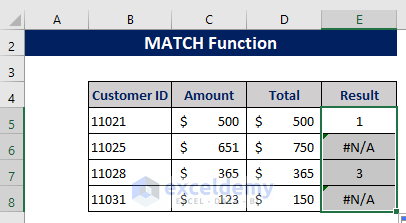
Method 3 – Insert MATCH Function to Find Value in a Column in Excel
Steps:
- We added a column Result to show the different function results.
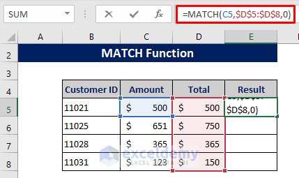
- Copy this formula in Cell E5:
=MATCH(C5,$D$5:$D$8,0)This find the value of Cell C5 in Column E of the range D5 to D8. Here we used the absolute sign so that the cell reference does not change. The last argument has been used as 0, as we want to get the exact result. This results in comparing Column C values on Column D.
- Press Enter.
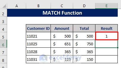
- We get 1 in Column E. It means our cell value is in the 1st position of our selected range.
- Use Fill Handle to autofill the entire column and we will get the positions if the values of Column C are found on Column D.
If we want to see TRUE or FALSE instead of position, we will need to apply the following steps:
- Apply this function to Cell E5:
=ISERROR(MATCH(C5,$D$5:$D$8,0))- Use Fill Handle from Cell E5.
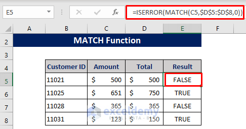
This shows whether the function encountered an error, so it’s displaying the opposite values. Wrap the formula in a NOT function to correct it.
- Edit the formula into:
=NOT(ISERROR(MATCH(C5,$D$5:$D$8,0)))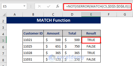
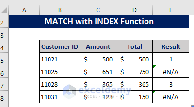
Method 4 – Link INDEX with MATCH Function to Find Value in a Column
Steps:
- Use the MATCH function from the previous method.
- Go to Cell E5 and edit the formula bar.
- Edit the formula into:
=INDEX(D5:D8,MATCH(C5,$D$5:$D$8,0))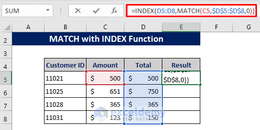
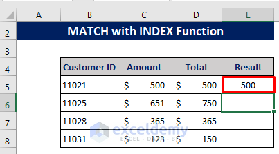
- Press Enter. The result is shown in the following image.
To show results in the rest of the cells, we have to autofill the rest of the cells in Column E.
- Edit the formula and use Absolute Reference:
=INDEX($D$5:$D$8,MATCH(C5,$D$5:$D$8,0))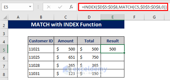
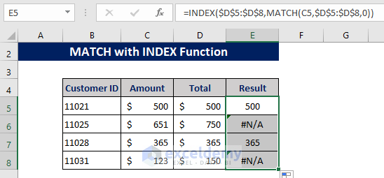
- Drag down the Fill Handle icon up to the last cell in Column E.
- The final output is shown in the following image.
Download Practice Workbook
Download this practice workbook to exercise while you are reading this article.
Related Articles
- How to Find First Value Greater Than in Excel
- How to Find First Occurrence of a Value in a Range in Excel
- Find Last Value in Column Greater than Zero in Excel
- How to Find First Occurrence of a Value in a Column in Excel
- How to Find Last Occurrence of a Value in a Column in Excel
<< Go Back to Find Value in Range | Excel Range | Learn Excel
Get FREE Advanced Excel Exercises with Solutions!
