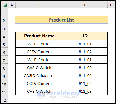
We will use the following dataset to explain formulas to find the first occurrence of a value in a range in Excel. The dataset contains two columns with the “Product Name“ and “ID“ of the products where you can notice repetitions of the values in the columns. Now, we need to find the first occurrence of a value in the range and explain three different formulas to do this.
Method 1 – Using COUNTIF or COUNTIFS Functions
Case 1.1 Utilizing COUNTIF Function
Steps:
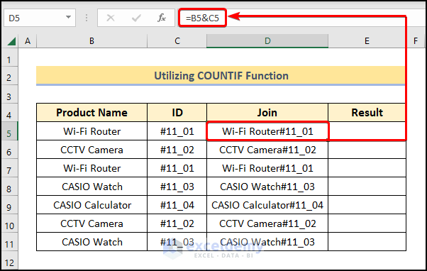
- Enter the formula given below into the D5 cell:
=B5&C5
- Press Enter.
- Drag the Fill handle icon to the other cells in the column.
- In E5, write the formula shown below:
=(COUNTIF($D$5:$D5,$D5)=1)+0- Hit Enter and drag the formula accordingly to get the result for all the rows.
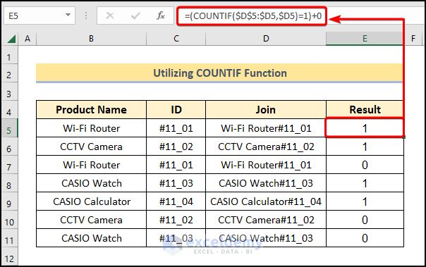
The result shows 1 for the values of the first occurrence in the range of cells D5:D11.
Note: Instead of adding zero we can use N Function nested with COUNTIF to get the same result.
Read More: How to Find First Occurrence of a Value in a Column in Excel
Case 1.2 Implementing COUNTIFS with N Function
Steps:
- Copy and paste this expression into the D5 cell:
=N(COUNTIFS(B$5:B5,B5,C$5:C5,C5)=1)- COUNTIFS(B$5:B5,B5,C$5:C5,C5) → counts the number of cells specified by a given set of conditions and criteria. Here, the B$5:B5 cells represent the criteria_range1 argument that refers to the “Product Name”, whereas the B5 cell indicates the criteria1 argument. Then, the C$5:C5 cells represent the criteria_range2 argument that refers to the “ID”, whereas the C5 cell indicates the criteria2 argument.
- Output → 1
- N(COUNTIFS(B$5:B5,B5,C$5:C5,C5)=1) → converts a non-number value to a number.
- Output → 1
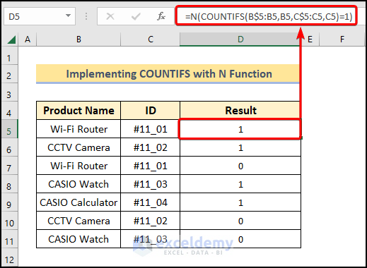
The result will be the same as Method 1.1.
The formula is the same as the method. The only difference is that here we do not need a join column. Again, COUNTIFS can take multiple ranges and criteria.
Method 2 – Applying Nested ISNUMBER and MATCH Functions
Steps:
- Type in this equation in cell D5:
=1- ISNUMBER(MATCH(B5,B$4:B4,0))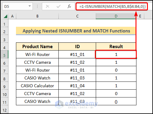
The result shows 1 for the first occurrence of the values in the range.
- MATCH(B5,B$4:B4,0) → returns the relative position of an item in an array matching the given value. Here, B5 is the lookup_value argument that refers to the Wi-Fi Router. Following, B$4:B4 represents the lookup_array argument from where the value is matched. Lastly, 0 is the optional match_type argument which indicates the Exact match criteria.
- Output → #N/A
- ISNUMBER(MATCH(B5,B$4:B4,0)) → checks whether a value is a number and returns TRUE or FALSE. Here, MATCH(B5,B$4:B4,0) is the value argument, and it returns FALSE.
- Output → FALSE
- 1-FALSE → 1
Method 3 – Employing Nested INDEX with other Functions
Case 3.1 Using Nested INDEX and MATCH Functions
Steps:
- The formula for the given dataset will be:
=INDEX($C$5:$C$11,MATCH($B$5,$B$5:$B$11,0))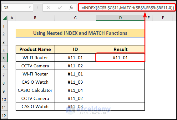
The result shows the value of Cell C5 with the first occurrence of the value of Cell B5 in the range B5:B11.
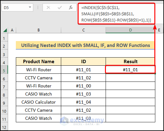
Case 3.2 Utilizing Nested INDEX with SMALL, IF, and ROW Functions
Steps:
- The formula is:
=INDEX($C$5:$C$11,SMALL(IF($B$5=$B$5:$B$11,ROW($B$5:$B$11)-ROW($B$5)+1),1))- IF($B$5=$B$5:$B$11,ROW($B$5:$B$11)-ROW($B$5)+1) → checks whether a condition is met and returns one value if TRUE and another value if FALSE. Here, $B$5=$B$5:$B$11 is the logical_test argument while the function returns ROW($B$5:$B$11)-ROW($B$5)+1 (value_if_true argument) otherwise it returns (value_if_false argument).
- SMALL(IF($B$5=$B$5:$B$11,ROW($B$5:$B$11)-ROW($B$5)+1),1) → returns the kth smallest value in data set.
- Output → 1
- INDEX($C$5:$C$11,SMALL(IF($B$5=$B$5:$B$11,ROW($B$5:$B$11)-ROW($B$5)+1),1)) → returns a value at the intersection of a row and column in a given range. In this expression, the $C$5:$C$11 is the array argument. Next, SMALL(IF($B$5=$B$5:$B$11,ROW($B$5:$B$11)-ROW($B$5)+1),1) is the row_num argument that indicates the row location.
- Output→ “#11_01”
Further, the result will be the same as Method 3.1 of this section.
- With this formula, you can also get the value of the 2nd time occurring value in the range by changing the 1 at the end of the formula by 2.
- Let’s change the ID number for the 2nd occurred “Wi-Fi Router” value to “#11_00″.
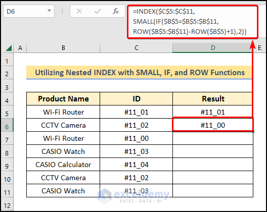
- At this point, the result shows “#11_00” which is the ID number of the 2nd time-occurring of the value “Wi-Fi Router” in the range.
Case 3.3 Applying Nested INDEX with ISNUMBER & SEARCH Functions for Duplicates Only
Steps:
- Select cell D5 and insert the formula as shown below:
=INDEX($E$5:$E$7,MATCH(TRUE,ISNUMBER(SEARCH($E$5:$E$7,B5)),0))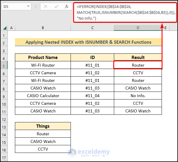
In addition, you can notice that the output at Cell D9 shows invalid results. It is because it has no duplicates within the range.
How to Find Last Occurrence of a Value in a Column in Excel via XLOOKUP
Steps:
- Enter the formula given below into the G5 cell:
=XLOOKUP(G4,C5:C12,D5:D12,,,-1)
Here, the C5:C12 and D5:D12 cells refer to the “Item” and “Price” columns.

Admittedly, we’ve skipped other relevant examples of how to find the last occurrence of a value in Excel, which you may explore if you wish.
Things to Remember
- Firstly, use the Fill handle icon to drag the formula for finding results for the rest of the values in the range.
- Second, you have to understand how you want your result and then apply any of the methods which suit you.
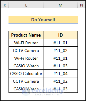
Practice Section
Additionally, we have provided a Practice section on the right side of each sheet so you can practice yourself. Please make sure to do it by yourself.
Download Practice Workbook
Related Readings
- How to Find Multiple Values in Excel
- How to Find First Value Greater Than in Excel
- Find Last Value in Column Greater than Zero in Excel
- How to Find Value in Column in Excel
<< Go Back to Find Value in Range | Excel Range | Learn Excel
Get FREE Advanced Excel Exercises with Solutions!
