In Excel 2019 or earlier versions, when using array formulas, press Ctrl + Shift + Enter instead of the Enter key and drag down the Fill Handle icon. For newer versions, press Enter. Here’s an overview of an array formula to fetch top 5 values.

Method 1 – How to Find the Top 5 Values and Names with Duplicates in Excel
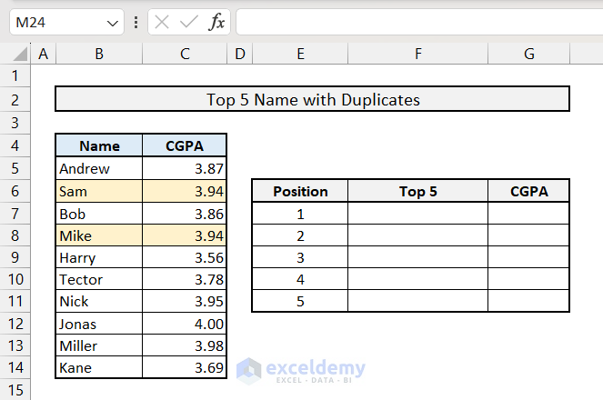
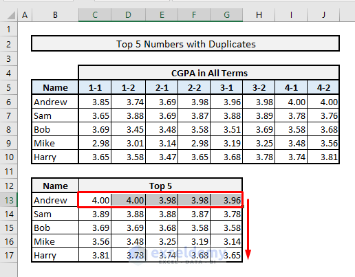
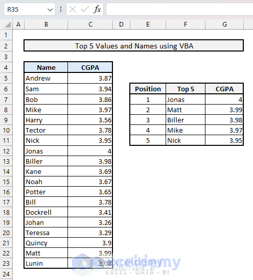
Column B represents random names of 10 students and Column C shows the CGPA of each student of a term final. Sam and Mike both have a similar CGPA, 3.94. We want to find the top 5 names.
Case 1.1 – Using a Combination of LARGE, ROWS, INDEX, MATCH, LARGE, COUNTIF Functions
Steps:
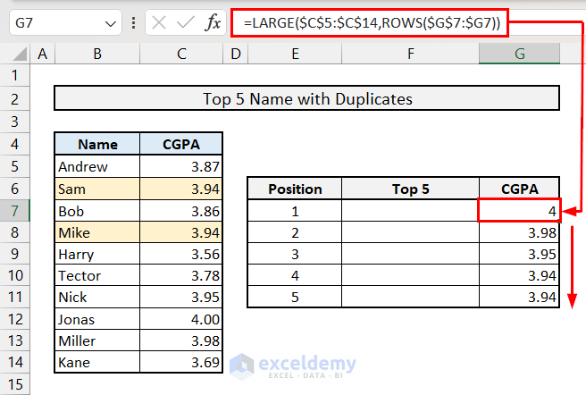
- In Cell G7, insert the following formula.
=LARGE($C$5:$C$14,ROWS($G$7:$G7))- Press the Enter key and drag down the Fill Handle icon to copy the formula in the remaining cells. This will calculate the top 5 values.
- Select Cell F7 and insert:
=INDEX($B$5:$B$14, MATCH(1, ($C$5:$C$14=LARGE($C$5:$C$14, $E7))*(COUNTIF(F$6:F6, $B$5:$B$14)=0), 0))- Press Enter and use the Fill Handle to get the other four names.
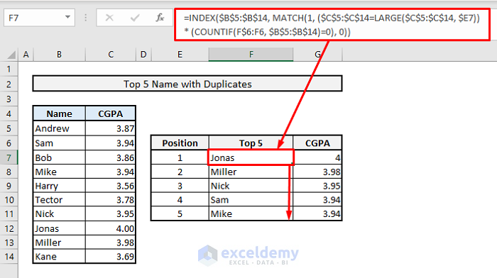
How Does This Formula Work?
- Inside the MATCH function, two logical functions are presented which are multiplied by each other. These combined logical functions will search for the top 5 CGPA from Column C and will assign the number 1 for the top 5 and 0 for the rest of the values.
- The MATCH function then searches for 1 only from the previous results found and returns the row numbers for all matches.
- The INDEX function finally shows the names serially based on those row numbers found through all MATCH functions in Column F.
Case 1.2 – Joining SORT, FILTER, and LARGE Functions
Steps:
- In Cell F7, the formula is:
=SORT(FILTER(B5:C14, C5:C14>=LARGE(C5:C14, 5)), 2,-1)- Press Enter.
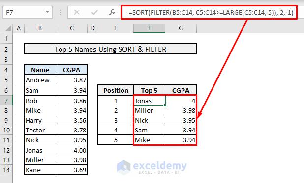
The FILTER function with the LARGE function inside extracts all the largest values from the Range of Cells- C5:C14. The SORT function then shows all the values or CGPA in descending order along with the names from the array of B5:C14.
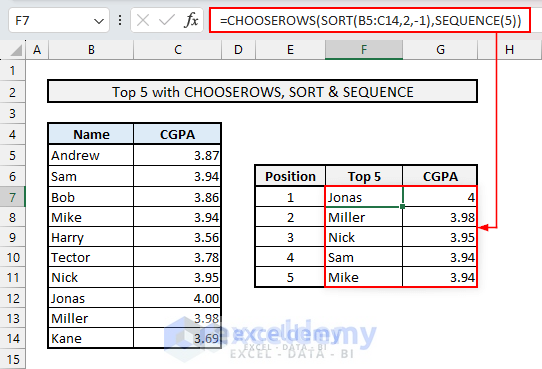
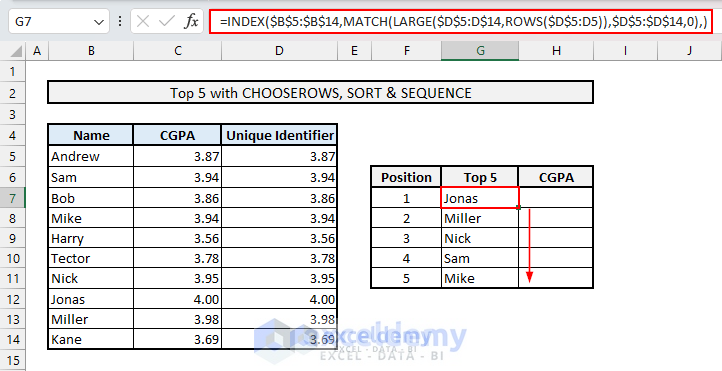
Case 1.3 – Combining CHOOSEROWS, SORT, SEQUENCE Functions
This formula is also only applicable in Excel for Microsoft 365 as the CHOOSEROWS function isn’t available in other versions.
Steps:
- Insert the following formula in Cell F7.
=CHOOSEROWS(SORT(B5:C14,2,-1),SEQUENCE(5))- Press the Enter key. The top 5 values and names will appear in the range F7:G11.
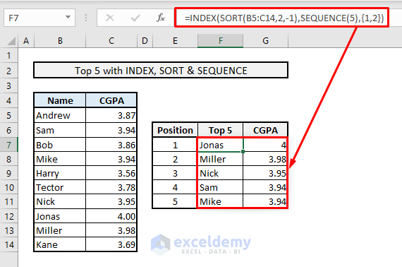
Case 1.4 – Using INDEX, SORT, and SEQUENCE Functions
Steps:
- Select Cell F7 and insert:
=INDEX(SORT(B5:C14,2,-1),SEQUENCE(5),{1,2})- Press Enter.
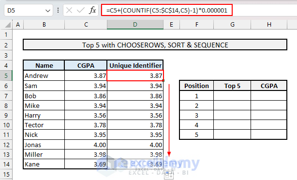
Case 1.5 – Finding the Top 5 Values and Names by Creating Unique Identifiers
Steps:
- We require an additional column Unique Identifier (column D) for this method. In Cell D5, insert the following formula.
=C5+(COUNTIF(C5:$C$14,C5)-1)*0.000001
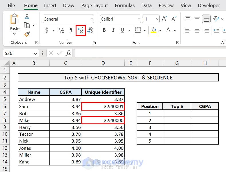
- Press the Enter key and drag down the Fill Handle icon.
- If you use the Increase Decimal button on the duplicates, you will notice that they are different now.
- Insert the formula below in Cell G7, then press the Enter key and use the Fill Handle tool to copy the formula down.
=INDEX($B$5:$B$14,MATCH(LARGE($D$5:D$14,ROWS($D$5:D5)),$D$5:$D$14,0),)This will find us the Top 5 names.
- For the top 5 values, insert the following formula in Cell H7 and press the Enter key, then drag down the Fill Handle icon.
=INDEX($C$5:$C$14,MATCH(LARGE($D$5:D$14,ROWS($D$5:D5)),$D$5:$D$14,0),)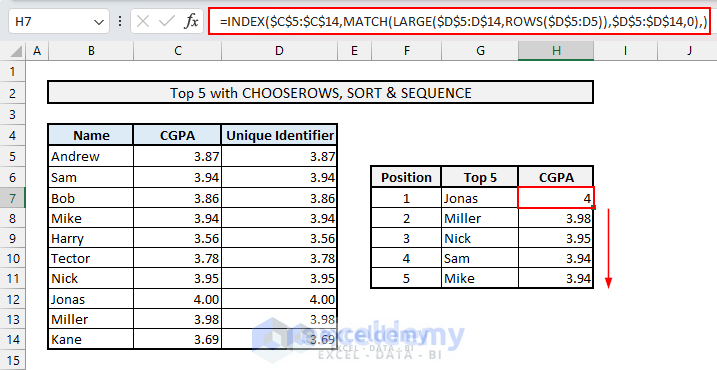
Case 1.6 – Using LARGE and COLUMNS Functions Together
Column B represents the names of 5 students and Columns C to J show the CGPA of each semester for those students. We’ll fetch the top 5 values for each student.
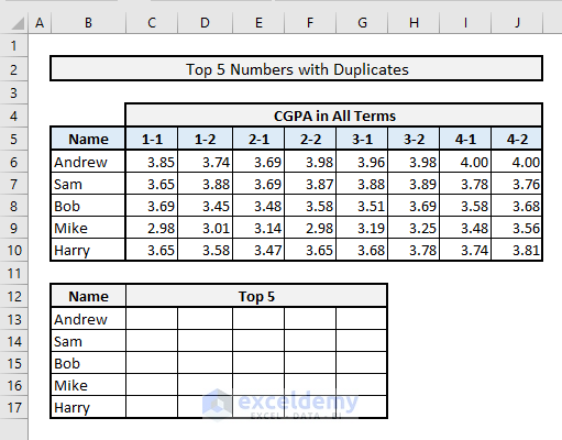
Steps:
- Select Cell C13 and insert:
=LARGE($C6:$N6,COLUMNS($C:C))- Press Enter and use the Fill Handle to fill the cells to the right.
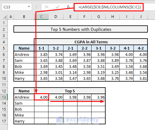
The LARGE function doesn’t omit duplicate values while searching for the largest ones from the range of data or cells.
- Select the range of cells C13:G13.
- Drag the Fill Handle down to fill all cells.
Read More: How to Create Top 10 List with Duplicates in Excel
Method 2 – How to Extract the Top 5 Values and Names without Duplicates in Excel
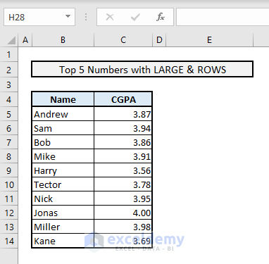
Case 2.1 – Getting the Top 5 Values by Using LARGE and ROWS Functions Together
We have a similar dataset as the previous section. However, no duplicates or ties are present in the dataset.
Steps:
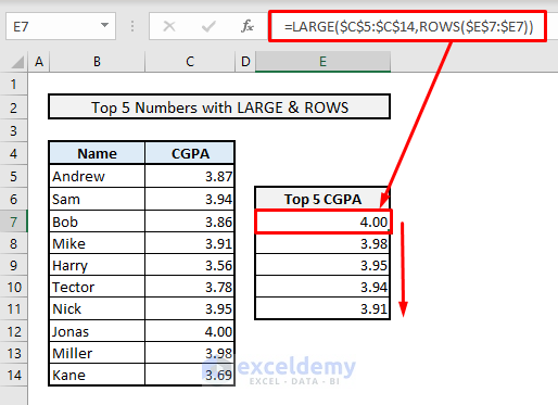
- Select Cell E7 and use the following formula.
=LARGE($C$5:$C$14,ROWS($E$7:$E7))- Press Enter.
- Use the Fill Handle to fill down.
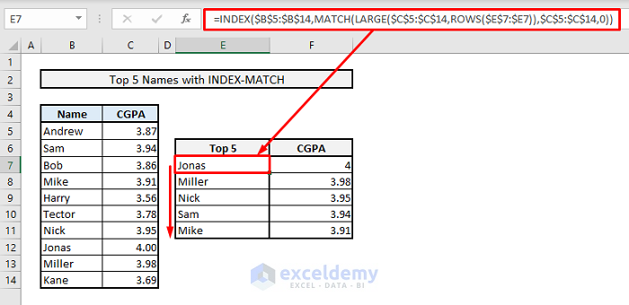
Case 2.2 – Find the Top 5 Names by Matching Top 5 Values
Option 1 – Using INDEX, MATCH, LARGE, and ROWS Functions Together
We’ll find out the names who got the top 5 CGPAs.
Steps:
- In Cell E7, the formula is:
=INDEX($B$5:$B$14,MATCH(LARGE($C$5:$C$14,ROWS($E$7:$E7)),$C$5:$C$14,0))- Hit Enter and you’ll get the first name ‘Jonas’ who got the highest CGPA- 4.00.
- Use the Fill Handle to fill down the column.
How Does This Formula Work?
- ROWS function inputs the serial number for the LARGE function.
- The LARGE function finds out the largest value from the array or range of cells selected based on the serial number.
- The MATCH function looks for the obtained largest value in the array of values & returns with the row number of that value.
- INDEX function finally pulls out the name from the column of Names based on that row number found by the MATCH function.
Option 2 – Combining XLOOKUP and LARGE Functions
Steps:
- In Cell E7, insert the following formula:
=XLOOKUP(LARGE($C$5:$C$14,ROWS($E$7:$E7)),$C$5:$C$14,$B$5:$B$14)- Press Enter and use the Fill Handle to get the other names.
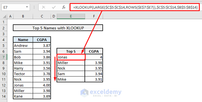
In the first argument of the XLOOKUP function, the largest value has been inputted. The second argument is the Range of Cells C5:C14 where the selected largest value will be looked for. The third argument is another range of cells B5:B14 from where the particular data or name will be extracted based on the row number found by the first two arguments.
Read More: Lookup Value in Column and Return Value of Another Column in Excel
Method 3 – How to Find the Top 5 Values and Names with Criteria in Excel
Case 3.1 – Finding the Top 5 Values and Names Based on a Single Criterion
Option 1 – Using INDEX, MATCH, LARGE, and IF Functions
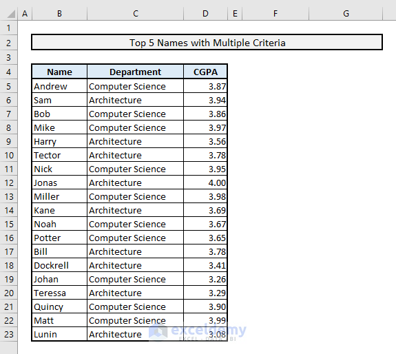
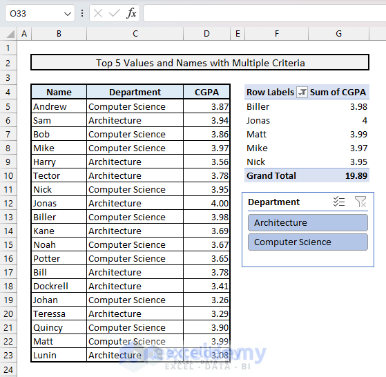
We have names and CGPA in Columns B and D respectively. Column C represents the departments of the students. We’ll find the top 5 CGPAs from the Computer Science department and store results in Column H.
Steps:
- To find the top 5 CGPAs, the related formula in Cell H12 will be:
=LARGE(IF($C$5:$C$23=$G$9,$D$5:$D$23),$F12)- Press Enter, then use the Fill Handle to get the other values.
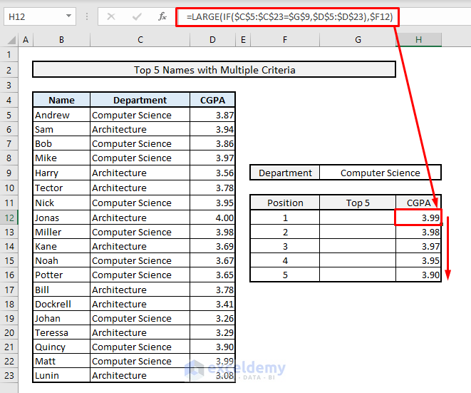
With the IF function, we’re finding out all the CGPAs of the students from the Computer Science department only. Then, the LARGE function extracts the top 5 CGPA like before.
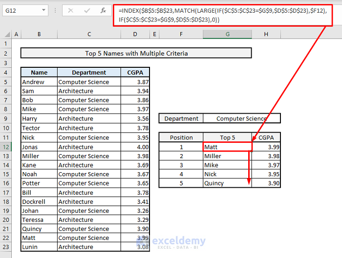
We’ll determine the names who got these top 5 CGPA’s and we’ll use INDEX-MATCH functions here.
Steps:
- In the output Cell G12, use:
=INDEX($B$5:$B$23,MATCH(LARGE(IF($C$5:$C$23=$G$9,$D$5:$D$23),$F12), IF($C$5:$C$23=$G$9,$D$5:$D$23),0))- Press Enter and use the Fill Handle to fill down the column.
Read More: How to Get Top 10 Values Based on Criteria in Excel
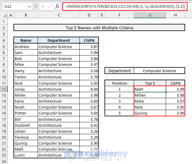
Option 2 – Applying INDEX, SORT, FILTER, and SEQUENCE Functions
If you are using Excel for Microsoft 365, then you can use a combination of INDEX, SORT, FILTER, and SEQUENCE functions.
Steps:
- Insert the following formula in Cell G12.
=INDEX(SORT(FILTER(B5:D23,C5:C23=G9),3,-1),SEQUENCE(5),{1,3})- Press the Enter key to get the list of the top 5 values and names.
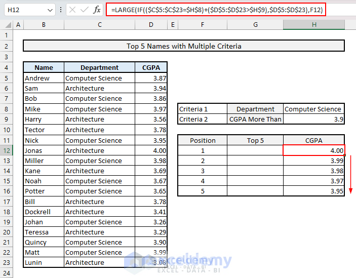
Case 3.2 – Finding the Top 5 Values and Names Based on Multiple Criteria
We want the top 5 names and values with Computer Science department criteria or a CGPA more than 3.9.
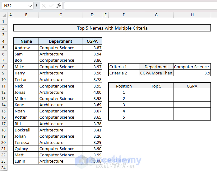
Steps:
- Insert the following formula in Cell H12 and press the Enter key, then drag down the Fill Handle icon.
=LARGE(IF(($C$5:$C$23=$H$8)+($D$5:$D$23>$H$9),$D$5:$D$23),F12)This will calculate the top 5 values.
- Use the following formula in Cell G12 and press the Enter key, then drag down or double-click the Fill Handle icon to get the top 5 names.
=INDEX($B$5:$B$23,SMALL(IF(($D$5:$D$23=H12)*(($C$5:$C$23=$H$8)+($D$5:$D$23>$H$9)),ROW($D$5:$D$23)-ROW($D$4)),COUNTIF(H12:$H$12,H12)))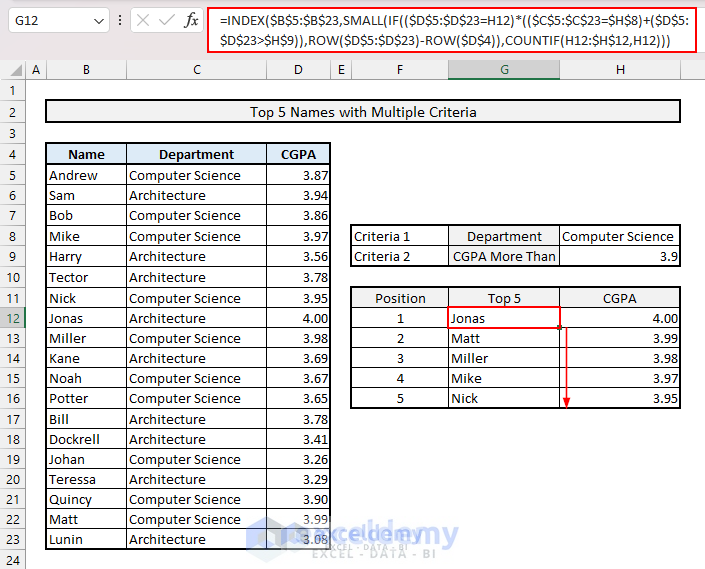
For the top 5 values with AND criteria, in Cell H12 apply the following formula:
=LARGE(IF(($C$5:$C$23=$H$8)*($D$5:$D$23>$H$9),$D$5:$D$23),F12)For the top 5 names with AND criteria, apply the following formula in Cell G12:
=INDEX($B$5:$B$23,SMALL(IF(($D$5:$D$23=H12)*(($C$5:$C$23=$H$8)*($D$5:$D$23>$H$9)),ROW($D$5:$D$23)-ROW($D$4)),COUNTIF(H12:$H$12,H12)))Case 3.3 – Inserting a Pivot Table Slicer to Find the Top 5 Values and Names Based on Criteria (Without Formula)
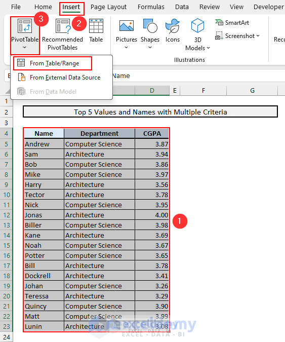
Steps:
- Select the range B4:D23.
- Go to the Insert tab.
- Click the PivotTable dropdown.
- Select the From Table/Range option.
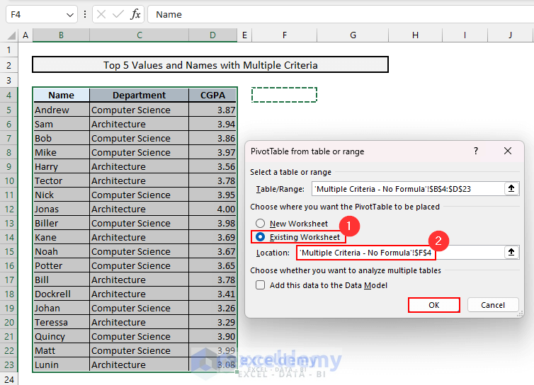
- A dialog box like will appear.
- Select the radio button of the Existing Worksheet option and set the Location to Cell F4.
- Click OK.
- A Pivot Table will appear in the selected location. The PivotTable Fields right-side pane will also appear.
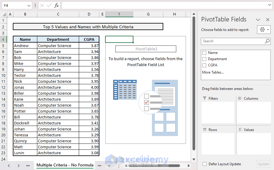
Click the image for a detailed view
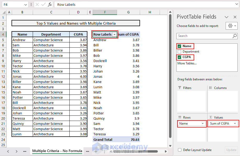
- Enable the checkboxes of Name and CGPA fields so that they appear in Rows and Σ Values areas, respectively.
- You will get a Pivot Table with Names as Row Labels and Sum of CGPA.
- There will be a dropdown icon for Row Labels.
Click the image for a detailed view
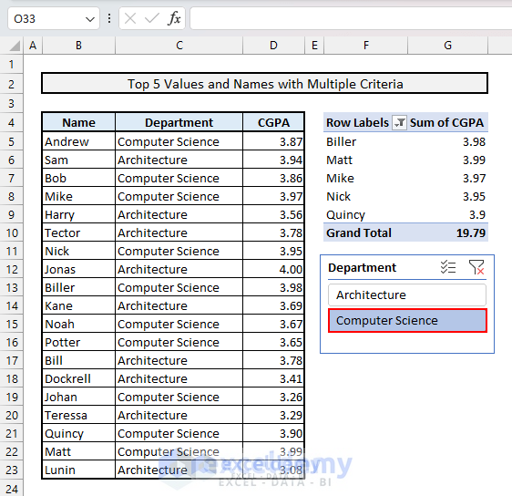
- Click the Row Labels dropdown and hover over the Value Filters option in the dropdown menu.
- Select the Top 10 option.
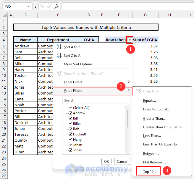
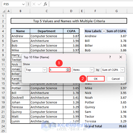
- You will get the Top 10 Filter (Name) dialog box.
- Reduce the number from 10 to 5.
- Click OK.
- Select any cell in the Pivot Table and you will find the PivotTable Analyze tab.
- Go to the PivotTable Analyze tab and you will find the Insert Slicer command.
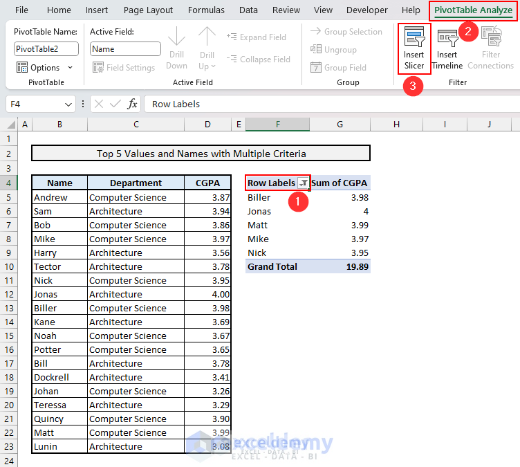
- You will get a dialog box. Check the Department box.
- Click OK.
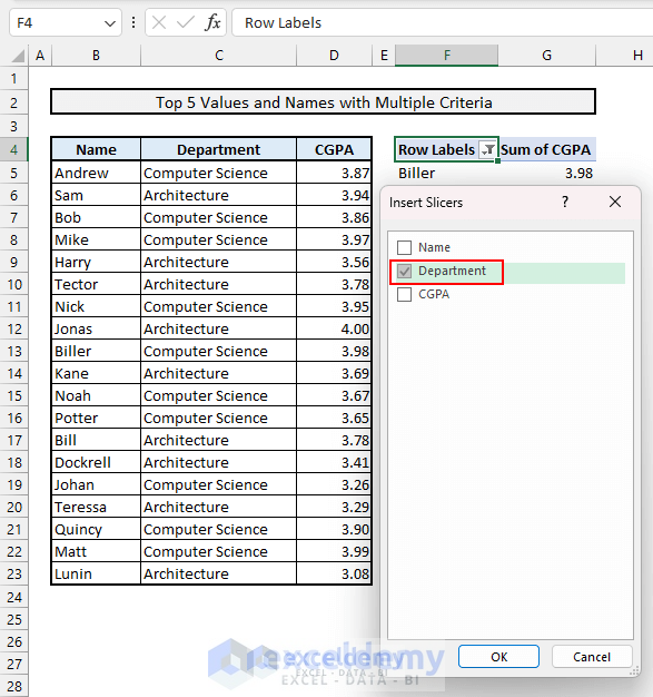
- The Department Slicer will appear in your worksheet.
- Select any department from the slicer.
- You will see the corresponding top 5 names and values in the Pivot Table.
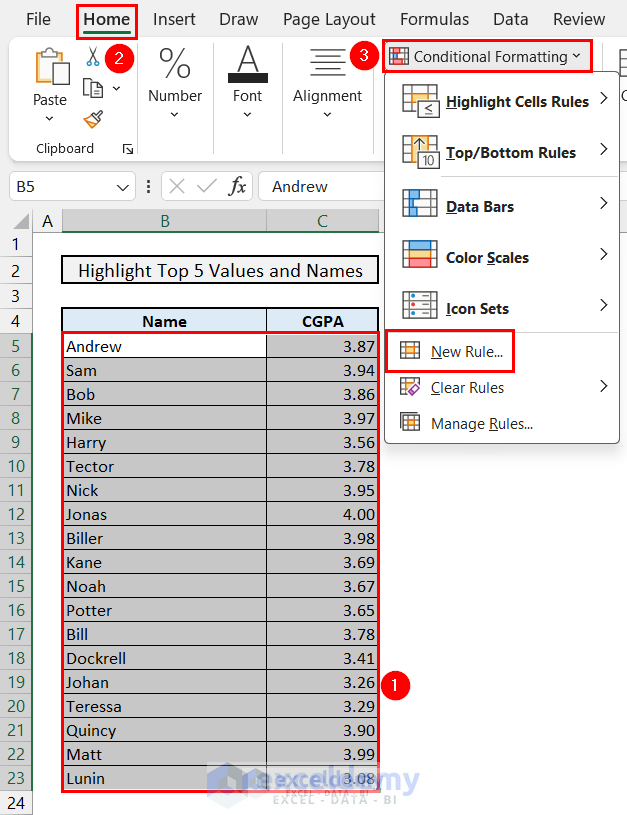
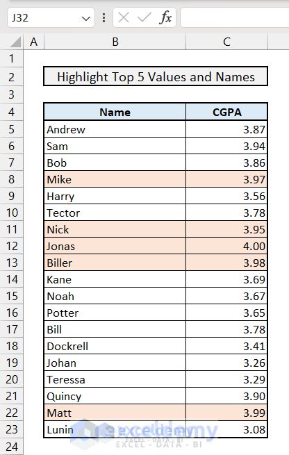
Method 4 – How to Highlight the Top 5 Values and Names Using Conditional Formatting in Excel
Steps:
- Select the range B5:C23.
- Go to the Home tab.
- Click on the Conditional Formatting dropdown.
- Select New Rule.
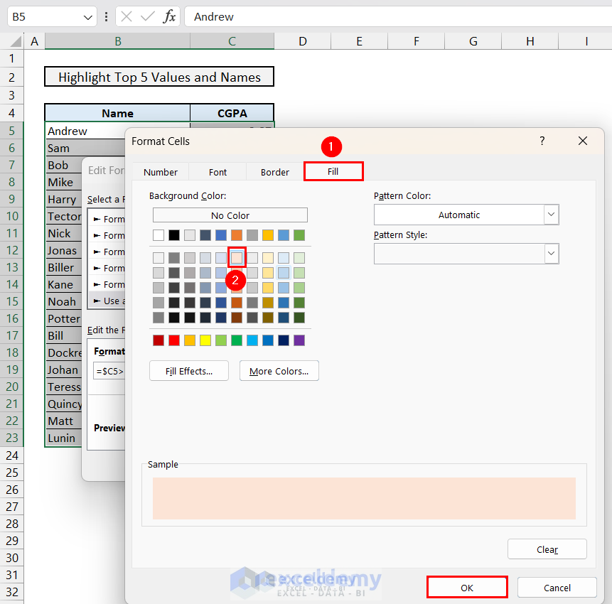
- You will get the Edit Formatting Rule dialog box.
- Select the Use a formula to determine which cells to format option.
- Set the formula to the following:
=$C5>=LARGE($C$2:$C$23,5)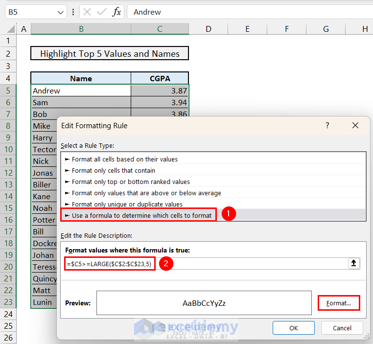
- Click the Format button and you will get the Format Cells dialog box.
- Go to the Fill tab and select the color you prefer.
- Click OK to go back to Format Cells.
Click the image to get a detailed view
- You will get a preview of the formatting of the formatted cells.
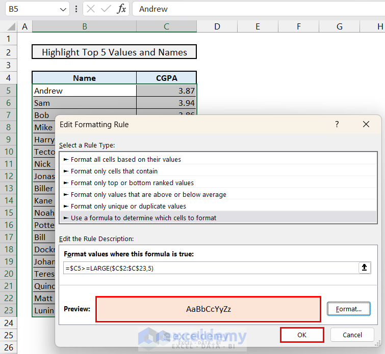
- Click the OK button in the Edit Formatting Rule dialog box.
- This will highlight the rows with the top 5 values and names.
Read More: How to Check If a Value is in List in Excel
Method 5 – How to Find the Top 5 Values and Names Using VBA
Steps:
- Go to the Developer tab.
- Select the Visual Basic option.
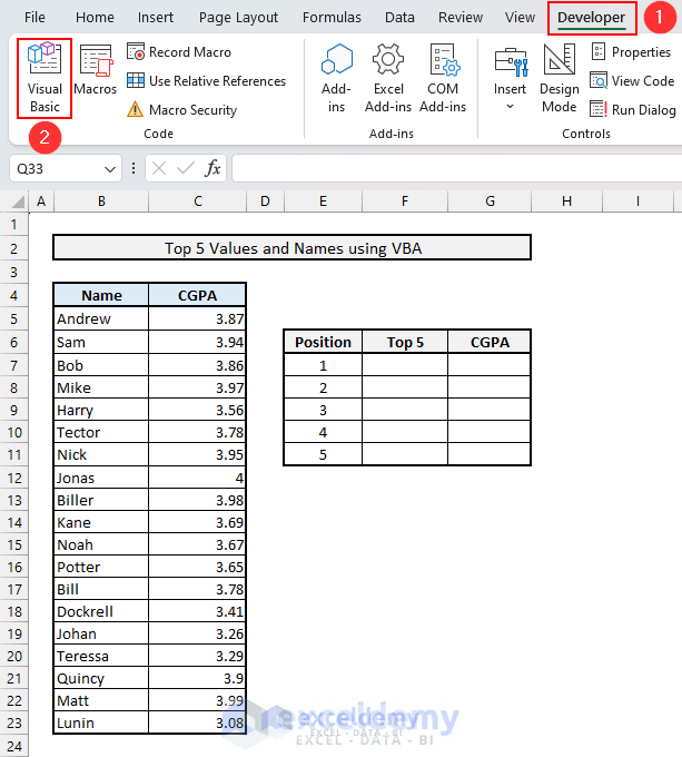
- The Visual Basic Editor window will open.
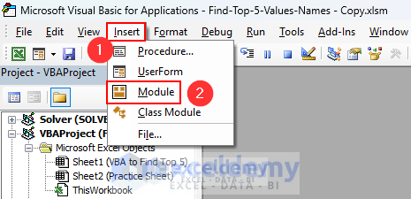
- Go to the Insert menu and select the Module option.
Note: If the Developer tab is not available in your Excel ribbon, you can use the keyboard shortcut Alt + F11 to open the Visual Basic Editor window.
- Module1 will appear.
- Insert the following code in the module.
- Click the Save button.
- Click the Run button.
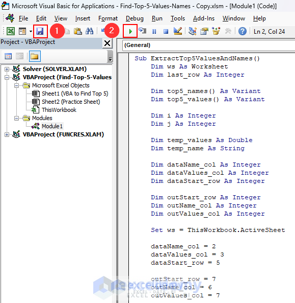
Sub ExtractTop5ValuesAndNames()
    Dim ws As Worksheet
    Dim last_row As Integer

    Dim top5_names() As Variant
    Dim top5_values() As Variant

    Dim i As Integer
    Dim j As Integer
    Dim k As Integer

    Dim temp_values As Double
    Dim temp_name As String

    Dim dataName_col As Integer
    Dim dataValues_col As Integer
    Dim dataStart_row As Integer

    Dim outStart_row As Integer
    Dim outName_col As Integer
    Dim outValues_col As Integer

    Set ws = ThisWorkbook.ActiveSheet

    dataName_col = 2
    dataValues_col = 3
    dataStart_row = 5

    outStart_row = 7
    outName_col = 6
    outValues_col = 7

    lastRow = ws.Cells(ws.Rows.Count, dataName_col).End(xlUp).Row

    ReDim top5_names(1 To 5)
    ReDim top5_values(1 To 5)

    For i = 1 To 5
        top5_values(i) = -1
    Next i

    For i = dataStart_row To lastRow
        temp_values = ws.Cells(i, dataValues_col).Value
        temp_name = ws.Cells(i, dataName_col).Value

        For j = 1 To 5
            If temp_values > top5_values(j) Then
                For k = 5 To j + 1 Step -1
                    top5_values(k) = top5_values(k - 1)
                    top5_names(k) = top5_names(k - 1)
                Next k

                top5_values(j) = temp_values
                top5_names(j) = temp_name
                Exit For
            End If
        Next j
    Next i

    For i = 1 To 5
        ws.Cells(i + outStart_row - 1, outName_col).Value = top5_names(i)
        ws.Cells(i + outStart_row - 1, outValues_col).Value = top5_values(i)
    Next i
End Sub- Return to your worksheet. You will find the top 5 values and names in the range F7:G11.
Things to Remember
- If you are using Excel 2019 or earlier versions, press Ctrl + Shift + Enter keys instead of the Enter key while using the array formulas.
- While imposing multiple criteria in the formula, use the Plus symbol (+) for OR logic and the Asterisk symbol (*) for AND logic.
- The list of top 5 values and names calculated using the Value Filters of Row Labels option in the Pivot Table is not sorted based on the values.
Download the Practice Workbook
Related Articles
- Find Text in Excel Range and Return Cell Reference
- How to Search Text in Multiple Excel Files
- [Solved!] CTRL+F Not Working in Excel
<< Go Back to Find Value in Range | Excel Range | Learn Excel
Get FREE Advanced Excel Exercises with Solutions!

Fantastic! What I was looking for.
Great examples. I am however looking for a way for the example in “1.4 Finding the Top 5 Names & Values under Multiple Criteria” to work with duplicate CGPA values. As it stands, if two or more NAMES in the same DEPARTMENT have the same CGPA values in the top 5, the solution in 1.4 will just repeat the first NAME in the list that appears with the duplicate CGPA value as many times as there are duplicate values. eg. If the highest CGPA value is 3.99 and shared by Andrew, Sam and Bob, the table will just list Andrew with 3.99 in Positions 1, 2 and 3 and never mention Sam or Bob. Is there a workaround?
I think your query should meet the requirements in methods 2.2 to 2.4. You can use any of them while dealing with similar numeric values. If it yet does not fulfill your criteria, then let me know. I’ll catch you up as soon as possible!
Hi,
First of, your solution really helped me. I ended up using the Index Match CountIF solution 2.2 for my worksheet and it worked for the queries I had upto 11 rows. However, I have an issue when i do a data set more that 11 rows as mentioned in your formulas in 2.2, it returns either an N/A error
Is there a way to increase the range of the row range?
The table range is with names in rows B2:B260, corresponding to a quantity column C2:C260 and a Net Column D2:D260. I have to pull out the best 5 and the worst 5 from the dataset.
Hello, we are glad to hear that our article has helped you. After seeing your comment, I have extended the dataset to 260 rows and the formulas have worked perfectly from my end. Can you please recheck whether you have changed the formula text corresponding to your dataset? For example, in the dataset of 11 rows the formula for largest 5 values will be like
=LARGE($C$5:$C$14,ROWS($G$7:$G7))but when you extended the dataset till 260th row then the formula will be like
=LARGE($C$5:$C$260,ROWS($G$7:$G7)).If you still face the problem then inform us in the reply. Thank you!
I used the Vlookup (1.3) method and it has worked, however it only shows the first column of my data not the second. Using Fill just repeats the same data. On 1.3 above i’m getting the right order for the names, but the CPGA isn’t showing. Any idea on how to correct it?
Thanks!
Hello RJ LENNOX!
In method 1.3m there have been shown only the formula for the names of the right order and in previous methods, there has been shown formula to get the value of CGPA in the right order. Please insert this formula into cell F7:
=LARGE($C$5:$C$14,ROWS($F$7:$F7))and, drag the fill handle to get the top 5 cgpa values.
I hope, your problem will be solved in this way. If not, please share the Excel file and send us the problem with a little more explanation in an email at [email protected]
Thank You!