We’ll use a dataset with student Names and marks in Physics, Chemistry and History. Note that this article uses Excel 365. Some functionalities may be missing in older Excel versions.
Method 1 – Find Top 10 Values Based on a Single Criterion in Excel
Case 1.1 – Insert a Combination of LARGE, IF, and ROW Functions
Let’s calculate the top 10 marks in physics for students who have more than 60 in chemistry.
- Select Cell G6 and insert the following formula there.
=LARGE(IF(D6:D20>60,C6:C20,""),ROW(A1:A10))- Press Enter.
- We will see the top 10 marks of physics in the range of cells G6:G15.
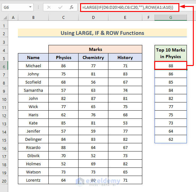
- ROW(A1:A10) creates an array of numbers 1 to 10.
- IF(D6:D20>60, C6:C20,””) checks the condition D6:D20>60, if the condition is met then it gives the output as a cell in the range of C6:C20, if criteria are not met it gives an empty value.
Case 1.2 – Apply XLOOKUP, LARGE, and FILTER Functions
Let’s extract the names of the students with the highest scores in Physics.
- Select Cell G6 and insert the following formula there.
=XLOOKUP(LARGE(FILTER(C6:C20,D6:D20>60),ROW(A1:A10)),C6:C20,B6:B20)- Hit Enter.
- We will see the Name of the students who got top 10 numbers in Physics.

- LARGE(FILTER(C6:C20,D6:D20>60),ROW(A1:A10)) gives the lookup value for the XLOOKUP function. The Filter function inside works same as the IF function.
- C6:C20 is the lookup_array and B6:B20 is the return_array.
Read More: How to Find Top 5 Values and Names in Excel
Case 1.3 – Use INDEX-MATCH Combination
Here’s an alternative that doesn’t use XLOOKUP.
- Select Cell G6 and write the following formula there.
=INDEX(B6:B20,MATCH(LARGE(FILTER(C6:C20,D6:D20>60),ROW(A1:A10)),C6:C20,0),1)- Press Enter.
- We will see the Names of students who got Top 10 Marks in Physics.
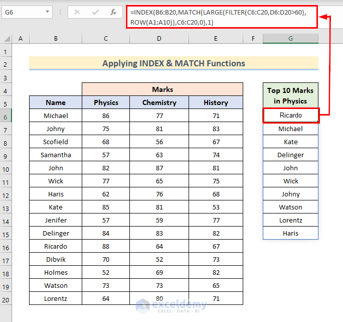
- ROW(A1:A10)) gives an array of 1 to 10.
- FILTER(C6:C20,D6:D20>60) checks the condition D6:D20>60 and gives output from C6:C20.
- The LARGE function takes the above parts as arguments and gives the output to 10 numbers.
Method 2 – Get Top 10 Values Based on Multiple Criteria in Excel
Let’s get the top 10 marks in physics that satisfy two conditions: the student has more than 50 in history and more than 60 in chemistry.
- Select Cell G6 and use the following formula there:
=LARGE(IF((--D6:D20>60)*(--E6:E20>50),C6:C20,""),ROW(A1:A10))- Hit Enter.
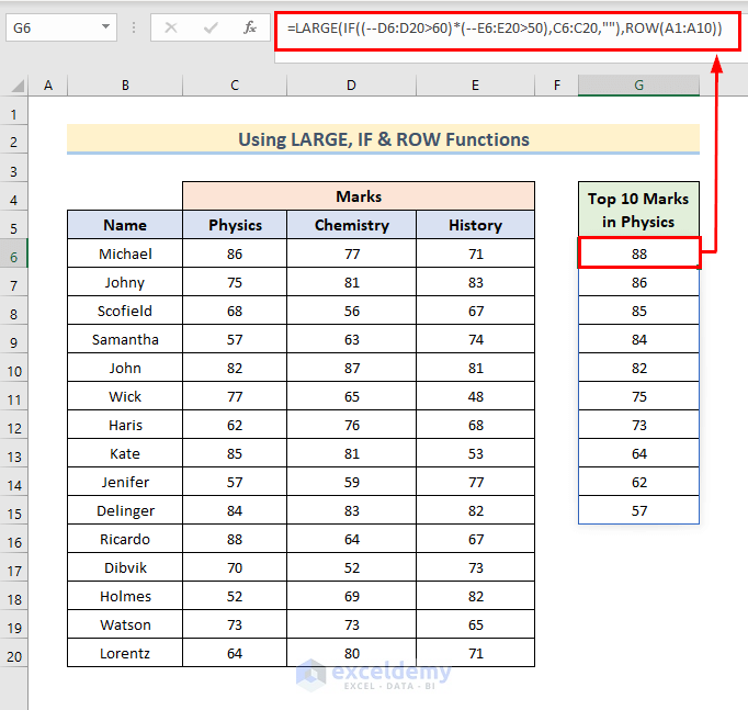
- ROW(A1:A10) creates an array of 1 to 10.
- IF((–D6:D20>60)*(–E6:E20>50),C6:C20,””) checks for the conditions and gives the output from the cell range C6:C20.
More Examples of Finding Top 10 Values in Excel
Example 1 – Use of the LARGE and ROW Functions to Get Top 10 Numbers
- Use the following formula:
=LARGE($C$6:$C$20,ROW(A1:A10))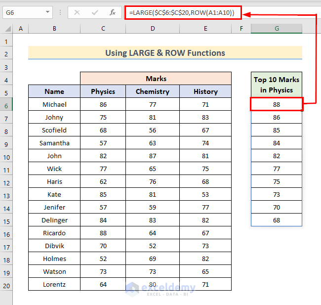
Note: The formula contains the LARGE and the ROW functions which work as described in the methods before.
Example 2 – Apply the LARGE and COLUMN Functions for Finding the Top 2 Values in a Row
- Insert the following formula in the first result cell and hit Enter.
=LARGE($C6:$E6,COLUMN(A1:B1))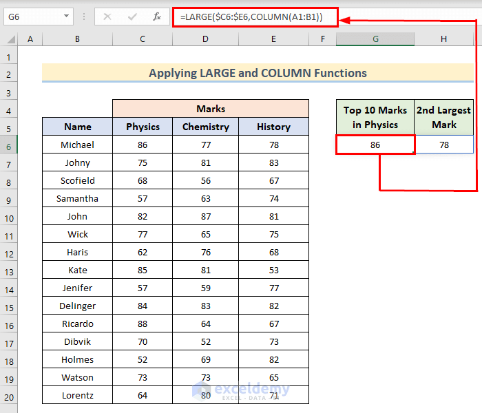
Note: The formula is similar to the previous example, except that it uses the COLUMN function (works along the row) instead of the ROW function.
Example 3 – Identify Top 10 Numbers Using the SORT and FILTER Functions
- Use the following formula for cell G6.
=SORT(FILTER(C6:C20,C6:C20>=LARGE(C6:C20,10)),1,-1)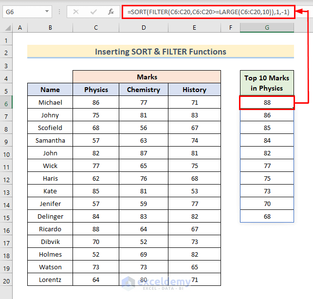
- FILTER(C6:C20,C6:C20>=LARGE(C6:C20,10)) finds the top numbers.
- The SORT function rearranges the numbers in descending order.
Example 4 – Utilize INDEX and MATCH Functions to Find Names That Correspond to Top 10 Values
- Select Cell G6 and enter the following formula:
=INDEX(B6:B20,MATCH(LARGE(C6:C20,ROW(A1:A10)),C6:C20,0),1)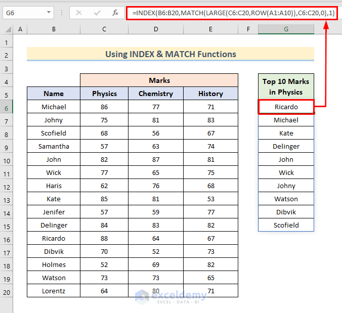
- B6:B20 is the reference number for the INDEX function.
- MATCH(LARGE(C6:C20,ROW(A1:A10)),C6:C20,0) gives the row number and 1 is the column number of the INDEX function.
Example 5 – Use XLOOKUP and LARGE Functions to Get the Top 10 Numbers
- Select Cell G6 and insert the following, then press Enter.
=XLOOKUP(LARGE(C6:C20,ROW(A1:A10)),C6:C20,B6:B20)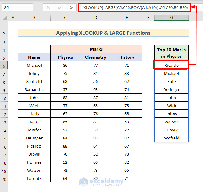
How to Identify Top 10 Values with Duplicates in Excel
- Select Cell G6 and insert the following formula there.
=LARGE(UNIQUE(E6:E20),ROW(A1:A10))- Hit Enter.
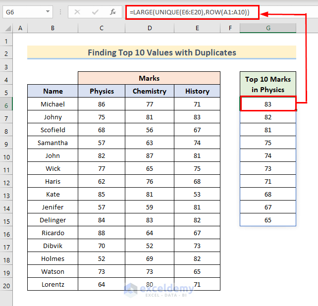
- UNIQUE(E6:E20) finds the unique values that act as the argument for other functions in the formula.
Read More: How to Create Top 10 List with Duplicates in Excel
Download the Practice Workbook
Related Articles
- How to Check If a Value is in List in Excel
- Lookup Value in Column and Return Value of Another Column in Excel
- Find Text in Excel Range and Return Cell Reference
- How to Search Text in Multiple Excel Files
- [Solved!] CTRL+F Not Working in Excel
<< Go Back to Find Value in Range | Excel Range | Learn Excel
Get FREE Advanced Excel Exercises with Solutions!

Great article. Congratulations
Many thanks
Hi Luis,
Thank you for your response. Hope this comes in handy for more people like you.
Great tool but let’s say that you have multiple students with the same mark in Physics. How would you return all their names? Xlookup only returns the first match for that score.
Thanks!
Hi Nico,
Thanks for your response. You can use the FILTER function of Excel for your problem. Check this article for details https://www.exceldemy.com/excel-filter-multiple-criteria/.
HELP!!!
Is there a way to look up the top 10 marks for all classes (cols C-E – so starting off with a top 10 table [Large(C6:E20,1), Large(C6:E20,2) and so on].
Then look up the class title and student name for each score… the issue I am finding is with the equal scores (for example, 77 comes up in several classes) – I cannot get it to show the student name & class for 1st instance of 77, or 2nd and so on.
Thanks for any help solving this!
Hey Philip,
Thanks for your response. You can use the SORT and FILTER functions along with the LARGE function to solve your problem.
Here’s the practice sheet we used. You can check it out for a better understanding.
SORT-FILTER.xlsx
You can also check out this article for more detailed explanations.
https://www.exceldemy.com/excel-top-10-list-with-duplicates/
Regards
Hassan Shuvo| ExcelDemy Team