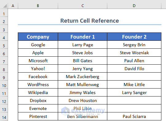
We will use the following dataset to return a cell reference based on a text value.
Method 1 – Use the INDEX and MATCH Functions to Find a Text in Range and Return a Cell Reference
We will search the text in a single column and the formula will return the reference to that cell.
Steps:
- Select cell D17 to keep the result.
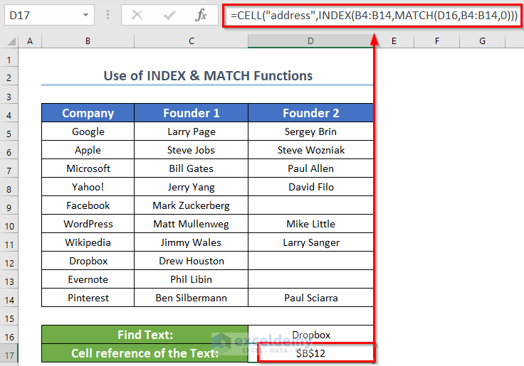
- Use the following formula in the D17 cell.
=CELL("address",INDEX(B4:B14,MATCH(D16,B4:B14,0)))- Press Enter to get the result.
How does this formula work?
- MATCH(D16,B4:B14,0), returns the value 9 because the position of Dropbox is ninth in the array B4:B14.
- The overall formula becomes:
=CELL(“address”,INDEX(B4:B14,9))
- The INDEX(B4:B14,9) part refers to cell reference B12. So, the formula becomes: =CELL(“address”,B12)
- =CELL(“address”,B12) returns an absolute reference of the cell B12.
- We get $B$12 as the output of the formula.
Note: INDEX(B4:B14,9) can return either the value or the cell reference. This is the beauty of the INDEX Function.
Method 2 – Applying INDEX, MATCH, and OFFSET Functions
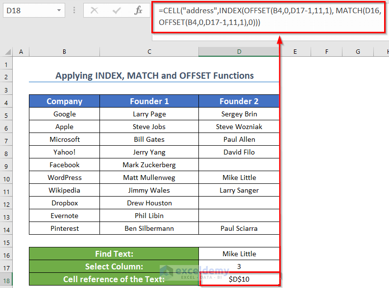
We will search for specific text (from D16) inside a specified column number (from D17) of the lookup array.
Steps:
- Use the following formula in the D18 cell.
=CELL("address",INDEX(OFFSET(B4,0,D17-1,11,1), MATCH(D16,OFFSET(B4,0,D17-1,11,1),0)))- Press Enter to get the result.
How does this formula work?
- The column is selected dynamically using Excel’s OFFSET function: OFFSET(B4,0,D17-1,11,1)
Method 3 – Use Combined Functions to Find a Text in Range and Return the Cell Reference
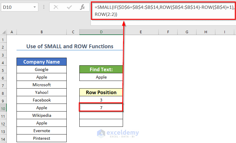
The text “Apple” is repeated 3 times in the range B4:B14. We’ll return all row numbers in the array.
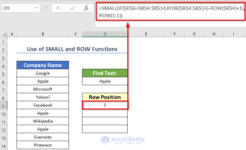
- Use this formula in cell D9.
{=SMALL(IF($D$6=$B$4:$B$14,ROW($B$4:$B$14)-ROW($B$4)+1),ROW(1:1))}- Insert this formula in the D10 cell.
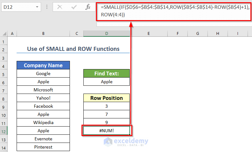
=SMALL(IF($D$6=$B$4:$B$14,ROW($B$4:$B$14)-ROW($B$4)+1),ROW(2:2))- Press Ctrl + Shift + Enter to get the result.
- We have copied the formula until the formula returns an error value.
The syntax of SMALL function:
SMALL(array,k)For example, SMALL({80;35;55;900},2) will return the 2nd smallest value in the array {80;35;55;900}. The output will be: 55.
How does the formula work?
Cell D9 = {=SMALL(IF($D$6=$B$4:$B$14,ROW($B$4:$B$14)-ROW($B$4)+1),ROW(1:1))}
To understand this array formula clearly, you can read our guide: 5 Examples of Using Array Formula in Excel
- IF($D$6=$B$4:$B$14,ROW($B$4:$B$14)-ROW($B$4)+1) returns the array for the SMALL function.
- Logical test part of the IF function is: $D$6=$B$4:$B$14. This part tests (one by one) whether the values of the range $B$4:$B$14 are equal to $D$6. If equal, a TRUE value is set in the array and if not equal, a False value is set in the array: {FALSE;FALSE;TRUE;FALSE;FALSE;FALSE;TRUE;FALSE;TRUE;FALSE;FALSE}
- ROW($B$4:$B$14)-ROW($B$4)+1) returns an array like this: {1;2;3;4;5;6;7;8;9;10;11} – {1} + 1 = {0;1;2;3;4;5;6;7;8;9;10} + 1 = {1;2;3;4;5;6;7;8;9;10;11}
- ROW(1:1) is actually the k of the SMALL function. And it returns 1.
- The formula in the cell D9 becomes like this: SMALL(IF({FALSE;FALSE;TRUE;FALSE;FALSE;FALSE;TRUE;FALSE;TRUE;FALSE;FALSE},{1;2;3;4;5;6;7;8;9;10;11}),1).
- The IF function returns this array: {FALSE;FALSE;3;FALSE;FALSE;FALSE;7;FALSE;9;FALSE;FALSE}.
- The formula becomes: SMALL({FALSE;FALSE;3;FALSE;FALSE;FALSE;7;FALSE;9;FALSE;FALSE},1).
- The formula returns 3.
Download the Working File
Related Articles
- How to Check If a Value is in List in Excel
- Lookup Value in Column and Return Value of Another Column in Excel
- How to Find Top 5 Values and Names in Excel
- How to Search Text in Multiple Excel Files
- [Solved!] CTRL+F Not Working in Excel
- How to Get Top 10 Values Based on Criteria in Excel
- How to Create Top 10 List with Duplicates in Excel
<< Go Back to Find Value in Range | Excel Range | Learn Excel
Get FREE Advanced Excel Exercises with Solutions!

I was wondering if there is a way to find part text with the above information to get reference cell?
There are 8 cell references to retrieve
There are blanks cells in range Z6 – Z270
DJ5 is the part cell reference
=SMALL(IF($DJ$5=$Z$6:$Z$270,ROW($Z$6:$Z$270)-ROW($Z$6)+1),ROW(1:1)) This returns 0 as not extract match
=CELL(“address”,INDEX(Z6:Z270,MATCH(DJ5,Z6:Z270,0))) This is a extract match & returns cell reference $Z$32
Is there a way to find part text from the above information?
There are 8 reference cells to retrieve.
There are blank cells in range Z6 – Z270
Reference part text cell DJ6
{=SMALL(IF($DJ$5=$Z$6:$Z$270,ROW($Z$6:$Z$270)-ROW($Z$6)+1),ROW(1:1))} Returns VALUE
=CELL(“address”,INDEX(Z6:Z270,MATCH(DJ5,Z6:Z270,0))) Returns extract match with extract cell reference $Z$32 only
=MATCH(DJ5&”*”,Z:Z,0)*1 Return extract cell row number 32.
All the above formula’s didn’t return 2 – 8 reference cells
Regards
Tony
Hi Tony,
I will check your formula.
Thanks.
Hi Kawser
I’m stump on the above information as to why I can’t get the information of the 8 reference’s & there cell reference.
Formula =MATCH(DJ5&”*”,Z:Z,0)*1 & add *2, *3, & so on for count
The reference part cell DJ5 = Track Time:
Track Time : refers to Conditions, Time & Fields
Regards
Tony