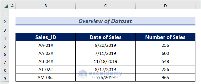
Lookup Value in Column and Return Value of Another Column in Excel

The sample dataset contains data related to the Sales_ID, the Date of Sales according to the ID number, and the Number of Sales that occurred for that particular ID number. We’ll extract data from a column and get the result of a different column.

Excel Lookup Value in Column and Return Value of Another Column

Method 1 – Use a LOOKUP Formula to Lookup a Value in a Column and Return a Value of Another Column

Apply the following formula in your result cell (i.e. C11) and press Enter.

=LOOKUP(B8,B5:B9,D5:D9)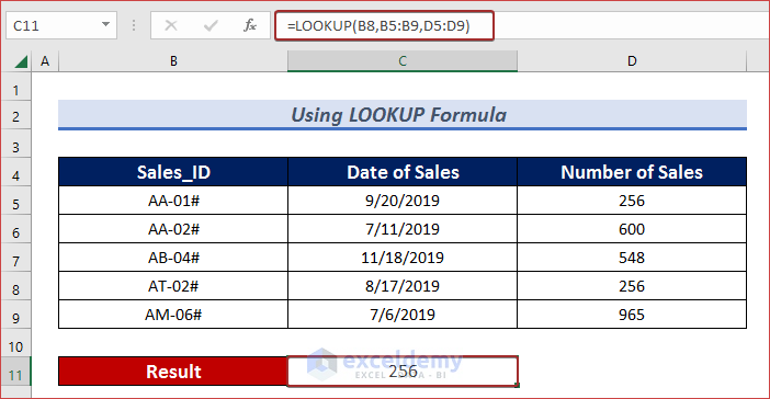

Use LOOKUP Formula to Lookup Value in Column and Return Value of Another Column

Method 2 – Use a VLOOKUP Formula to Lookup a Value in a Column and Return a Value of Another Column

Case 2.1 – VLOOKUP Formula for an Exact Match

Apply the following formula in your result cell (i.e. C11) and press Enter.

=VLOOKUP(B7,B5:D9,3, FALSE)

Case 2.2 – VLOOKUP Formula for a Partial Match

Apply the following formula in your result cell (i.e. C11) and press Enter.

=VLOOKUP("AA-03#",B5:D9,3,TRUE)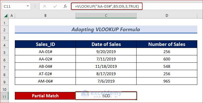

Method 3 – Combine VLOOKUP and IFERROR Functions to Lookup a Value in a Column and Return a Value of Another Column

Apply the following formula in your result cell (i.e. C11) and press Enter.

=IFERROR(VLOOKUP(B8,B5:D9,3,FALSE),"Not Found")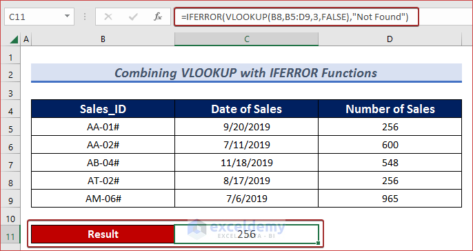

Method 4 – Merge INDEX and MATCH Functions to Lookup a Value in a Column and Return a Value of Another Column

Apply the following formula in your result cell (i.e. C12) and press Enter.

=INDEX(D5:D9,MATCH(B12,B5:B9,0))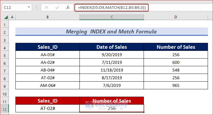

Formula Breakdown

MATCH(B12,B5:B9,0) —> finds the matched value location in range B5:B9.
Output: 4

INDEX(D5:D9,MATCH(B12,B5:B9,0))
INDEX(D5:D9,4)—> returns the fourth value in the range D5:D9.
Output: 256

Method 5 – Combine TEXTJOIN and IF Functions to Lookup a Value in a Column and Return a Value of Another Column

Apply the following formula in your result cell (i.e. C11) and press Enter.

=TEXTJOIN(", ",TRUE,IF(B12=B4:B9,D4:D9,""))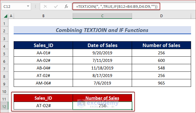

Download the Practice Workbook

Lookup Value in Column and Return Value of Another Column.xlsx