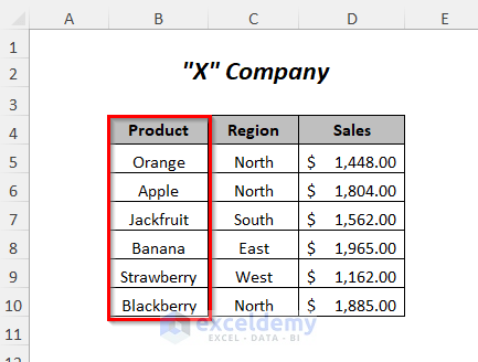
Consider a dataset about some products of a company. We will check whether specific values in the Product column exist.
Method 1 – Using Find & Select to Check If a Value Is in a List
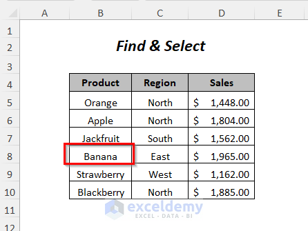
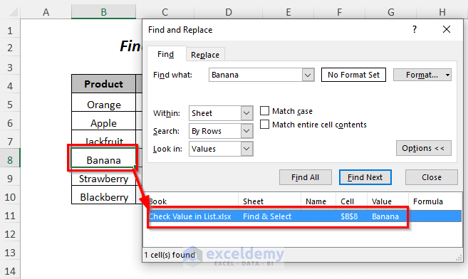
We are searching for the product Banana.
- Go to the Home tab, select Find & Select, and pick Find.
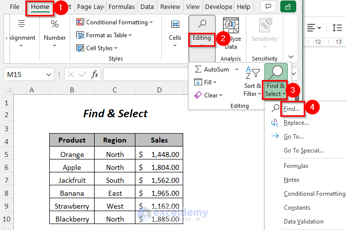
- The Find and Replace dialog box will appear.
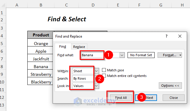
- Write down the name of the product you are looking for in the Find what box (Banana)
- Select the following: Within → Sheet; Search → By Rows; Look in → Values.
- Press Find All.
- You will get the cell positions of the product Banana in the list.
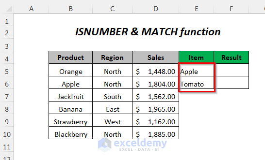
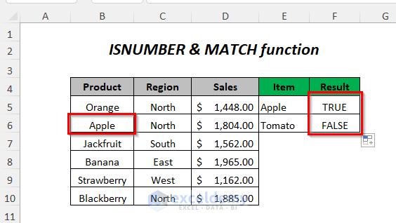
Method 2 – Using ISNUMBER and MATCH Functions to Check If a Value Is in a List
We have some items in the Item column which we want to check in the list of the products in the Product column. The check result will appear in the Result column.
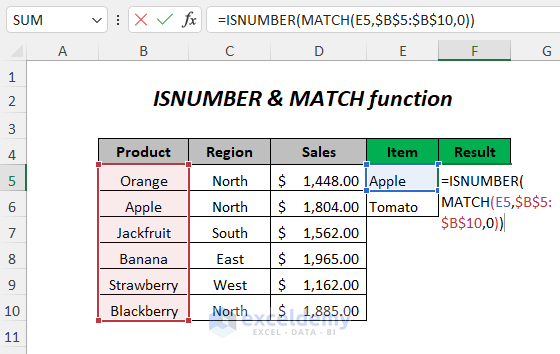
- Select the output cell F5.
- Insert the following formula:
=ISNUMBER(MATCH(E5,$B$5:$B$10,0))The MATCH function will return the position of the value in the E5 cell in the range $B$5:$B$10 if it is found. Otherwise, it will return #N/A. ISNUMBER will return TRUE if the value is a number (i.e. if MATCH finds something).
- Hit Enter and drag down the Fill Handle tool.
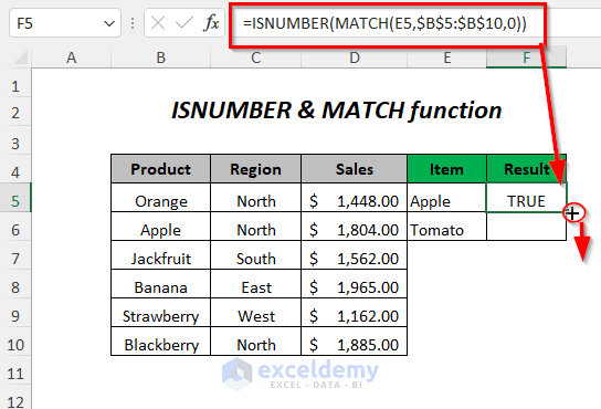
- Here are the results.
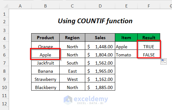
Method 3 – Using the COUNTIF Function
We’ll use the same conditions as in Method 2.
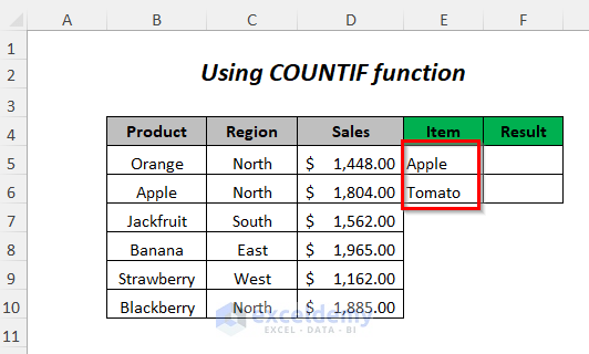
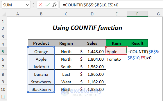
- Select the output cell F5.
- Insert the following formula
=COUNTIF($B$5:$B$10,E5)>0COUNTIF will return how many times the check value appears in the array, so it will be greater than 0 if it finds a result. The output will then be TRUE.
- Hit Enter and drag down the Fill Handle.
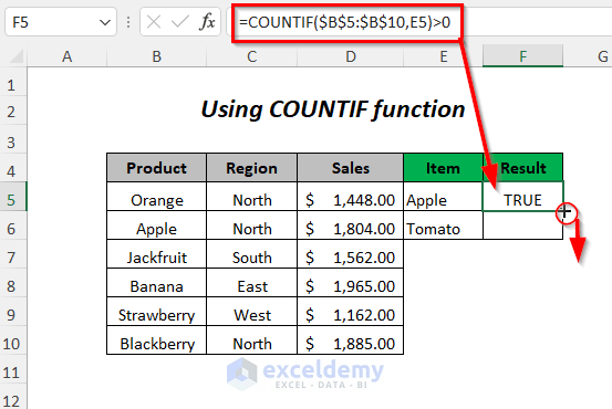
Results:
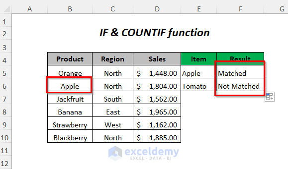
Method 4 – Using IF and COUNTIF Functions
We’ll use the same dataset as before.
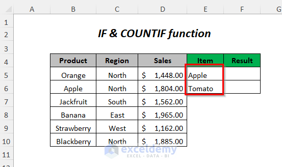
- Select the output cell F5.
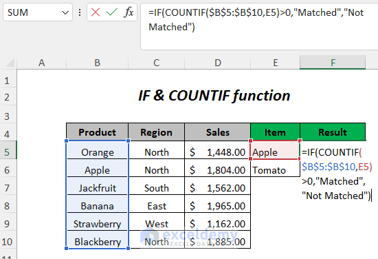
- Insert the following formula:
=IF(COUNTIF($B$5:$B$10,E5)>0,"Matched","Not Matched")$B$5:$B$10 is the range where you are checking your desired value and E5 is the value which you are looking for.
When COUNTIF finds the value in the list, it will return a number of occurrences of this value, so it will be greater than 0. IF will then return Matched. Otherwise, it will return Not Matched if the value is not in the list.
- Hit Enter and drag down the Fill Handle tool.
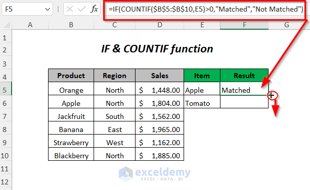
Results
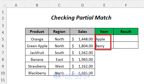
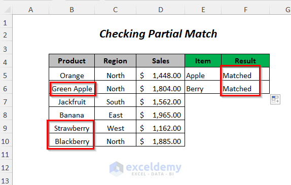
Method 5 – Checking a Partial Match with Wildcards
In the following table, we have Apple and Berry in the Item column but they are not exact matches to the product names (we have modified Apple in the dataset to Green Apple).
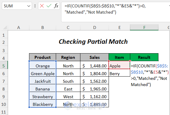
- Select the output cell F5.
- Insert the following formula:
=IF(COUNTIF($B$5:$B$10,"*"&E5&"*")>0,"Matched","Not Matched")E5 is the check value, where “*” is joined with this value by using the Ampersand operator. “*” is used to replace zero or more characters.
- Hit Enter and drag down the formula with the Fill Handle.
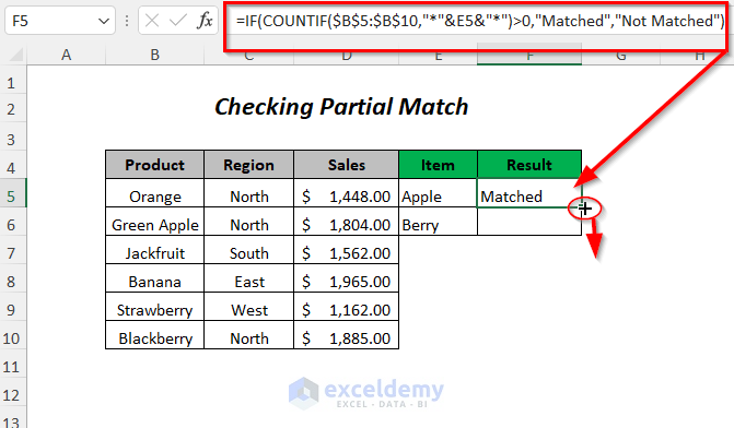
Results
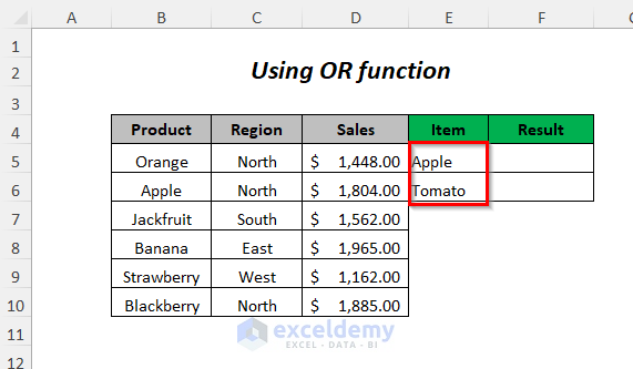
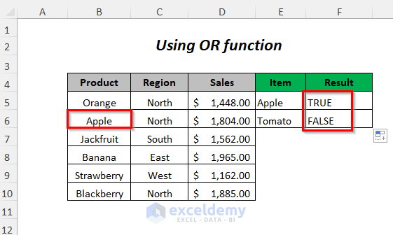
Method 6 – Using the OR Array Function to Check If a Value Is in a List
We’ll use the same dataset.
- Select the output cell F5.
- Insert the following formula:
=OR($B$5:$B$10=E5)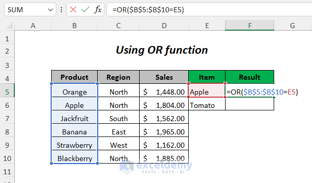
- Hit Enter and drag down the Fill Handle to fill the other cells. If you are using any version other than Excel 365, press Ctrl + Shift + Enter instead of pressing Enter.
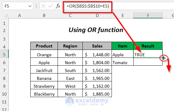
Results
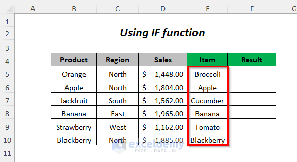
Method 7 – Using the IF Function to Check If Values in Lists Match
We’ll crosscheck two lists for matches across rows.
- Select the output cell F5.
- Insert the following formula:
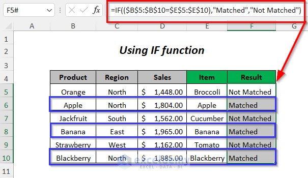
=IF(($B$5:$B$10=$E$5:$E$10),"Matched","Not Matched")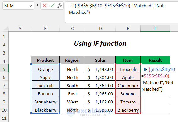
- Press Enter or Ctrl + Shift + Enter (for Excel versions other than Excel 365).
Results
Method 8 – Using the ISERROR and VLOOKUP Functions
We’ll go back to the base dataset and check item-wise.
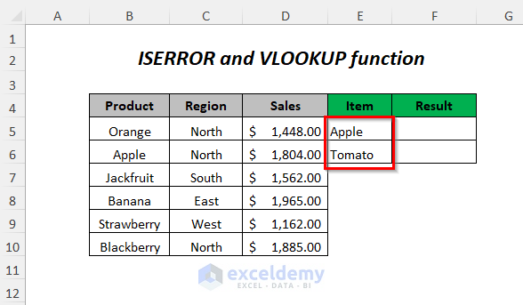
- Select the output cell F5.
- Insert the following formula:
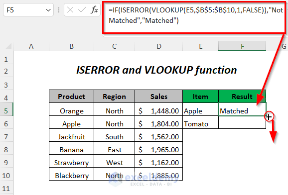
=IF(ISERROR(VLOOKUP(E5,$B$5:$B$10,1,FALSE)),"Not Matched","Matched")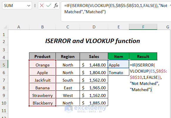
- Hit Enter and drag down the Fill Handle.
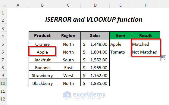
Results
Method 9 – Using ISERROR, INDEX, and MATCH Functions
We’ll use the same dataset as before.
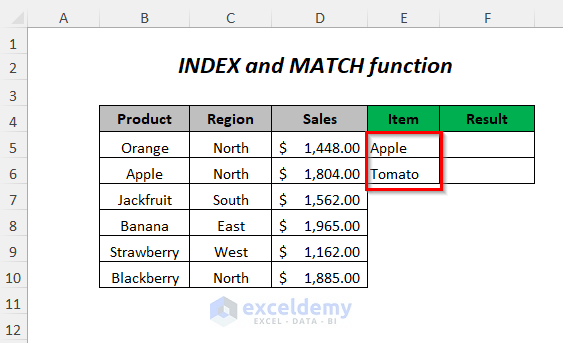
- Select the output cell F5.
- Insert the following formula:
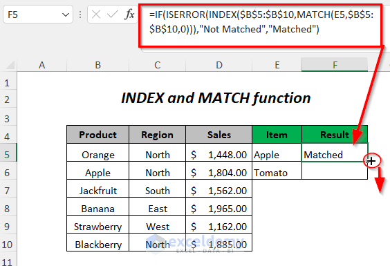
=IF(ISERROR(INDEX($B$5:$B$10,MATCH(E5,$B$5:$B$10,0))),"Not Matched","Matched")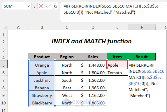
- Hit Enter and drag the Fill Handle down to fill other cells in the column.
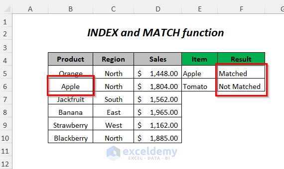
Results
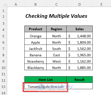
Method 10 – Checking Multiple Values in a List
We have a single cell that contains multiple values that may or may not be in the list. We’ll return the list of items that do appear in a list.
- Select the output cell D13.
- Insert the following formula:
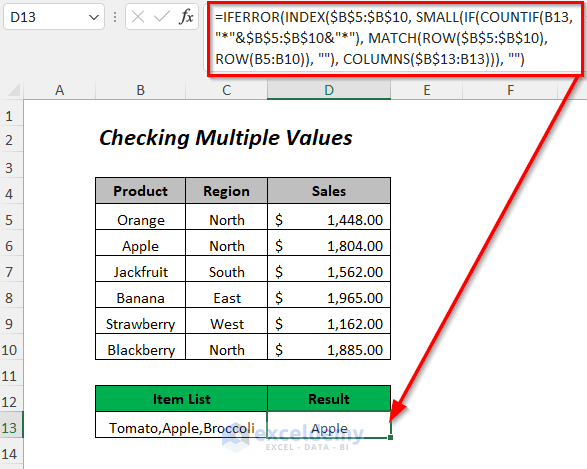
=IFERROR(INDEX($B$5:$B$10, SMALL(IF(COUNTIF(B13, "*"&$B$5:$B$10&"*"), MATCH(ROW($B$5:$B$10), ROW(B5:B10)), ""), COLUMNS($B$13:B13))), "")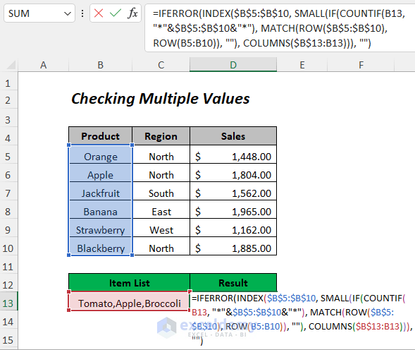
- Press Enter.
Results
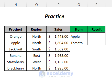
Practice Section
We have provided a Practice section like below for each method in each sheet.
Download the Practice Workbook
Further Readings
- Lookup Value in Column and Return Value of Another Column in Excel
- How to Find Top 5 Values and Names in Excel
- Find Text in Excel Range and Return Cell Reference
- How to Search Text in Multiple Excel Files
- [Solved!] CTRL+F Not Working in Excel
- How to Get Top 10 Values Based on Criteria in Excel
- How to Create Top 10 List with Duplicates in Excel
<< Go Back to Find Value in Range | Excel Range | Learn Excel
Get FREE Advanced Excel Exercises with Solutions!

METHOD 6: The use of OR in this context can be problematic in some edge cases because OR is not designed to handle array comparisons directly.
Hello Savoir-faire,
Thanks for pointing this out! Using OR with arrays can sometimes lead to unreliable results, especially in non-array formulas or older Excel versions. It’s better to use more robust methods like MATCH or COUNTIF, which handle list comparisons more efficiently and avoid edge cases where OR might fail. We used OR in this context is its simplicity and readability. For users working with Excel 365 or newer versions, this method provides an easy way to compare multiple values without needing complex functions like MATCH or COUNTIF. It’s particularly helpful for small datasets and straightforward checks. Additionally, the OR function works well for quick visual comparisons in smaller spreadsheets.
Regards
ExcelDemy
Thank you! I just used Method 2 and it was very handy.
Hello Guilherme Dellagustin,
You are most welcome. Thanks for your feedback and appreciation.
Keep exploring Excel with ExcelDemy!
Regards,
ExcelDemy