How to Filter by Color Using Conditional Formatting in Excel

While working in Excel, we often need to filter our data by color that is formatted by conditional formatting. Utilizing the conditional formatting feature of Excel, we can change the appearance of cells by applying various conditions. We can extract the specific data we want from a dataset by filtering the data according to color. We may be able to complete it manually if the dataset is small. However, manually filtering the data gets challenging for huge datasets. It turns into a time-consuming and tiresome activity. But you’re lucky! You live in a world where there is a program named Excel that contains solutions for practically every spreadsheet-related issue. With a few simple steps in Excel, we can filter our data by color that is formatted by conditional formatting.

How to Filter by Color Using Conditional Formatting in Excel: 3 Steps

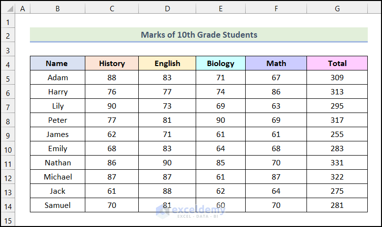
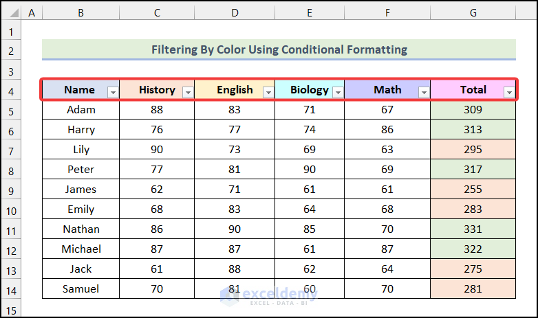
In this section of the article, we will learn 3 simple steps to filter our data by color that is formatted by conditional formatting. Let’s say we have Marks of 10th Grade Students of a school, and we want to filter the Total Marks based on 2 criteria. They are as follows.

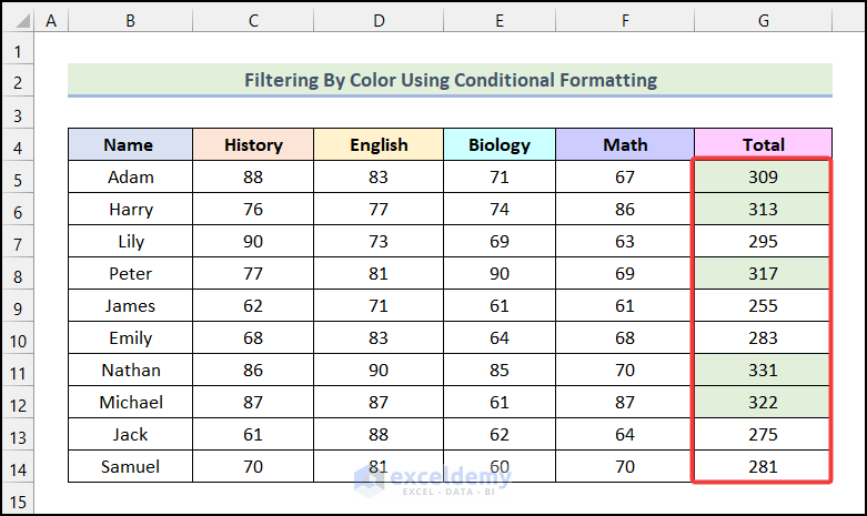
• Total > 299 → Format cell with a Green fill.
• Total < 300→ Format cell with a Red fill.

Let’s follow the steps mentioned below to do this.

Not to mention that we have used the Microsoft Excel 365 version for this article; you can use any other version according to your convenience.

Step 01: Apply Conditional Formatting First

In the first step, we need to apply conditional formatting to our data so that we can add different colored fill to the cells of the Total column based on the conditions mentioned before.

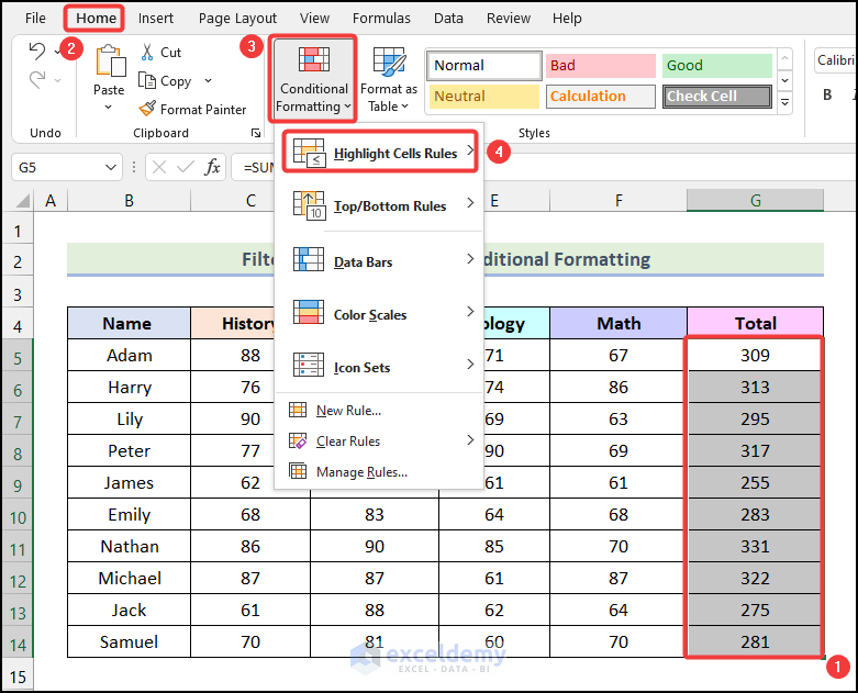
• Firstly, select the cells of the Total column as marked in the following image.
• Following that, go to the Home tab from Ribbon.
• Then, choose the Conditional Formatting option from the Styles group.
• After that, select the Highlight Cells Rules option from the drop-down.

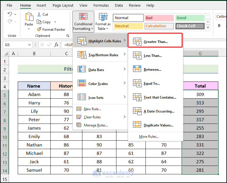
• Next, choose the Greater Than option as shown in the image below.

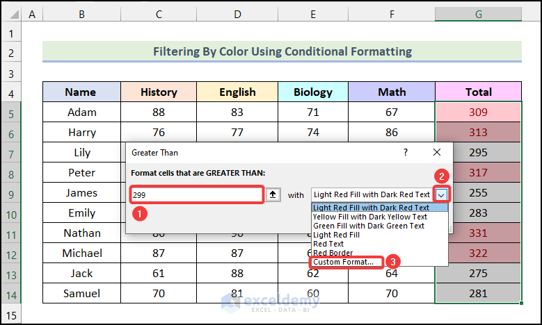
As a result, the Greater Than dialog box will open.

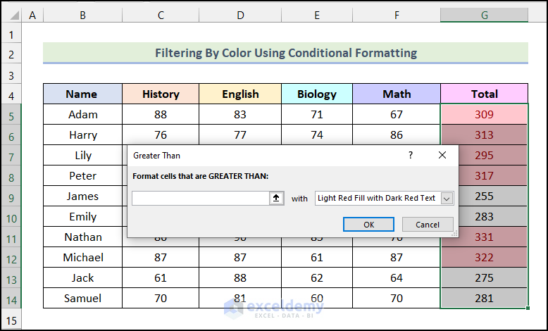
• Now, in the Greater Than dialog box, type 299 in the marked field.
• Following that, click on the drop-down icon and choose the Custom Format option from the drop-down.

Consequently, the Format Cells dialog box will be visible on your worksheet.

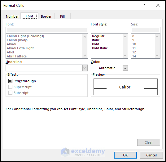
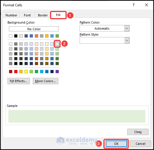
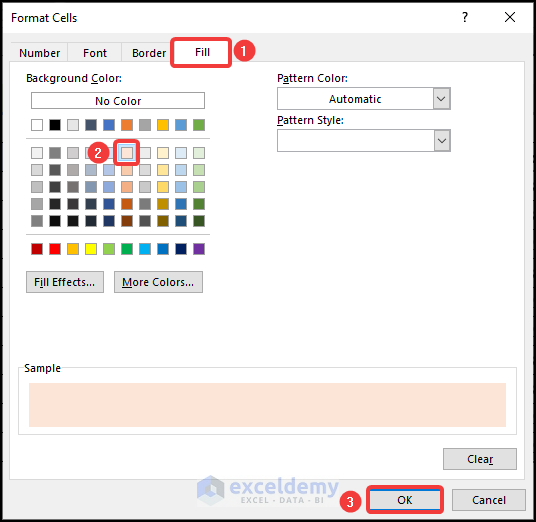
• After that, in the Format Cells dialog box, go to the Fill tab.
• Then, choose your preferred color.
• Subsequently, click on OK.

• As a result, you will be redirected to the Greater Than dialog box and click on OK there.

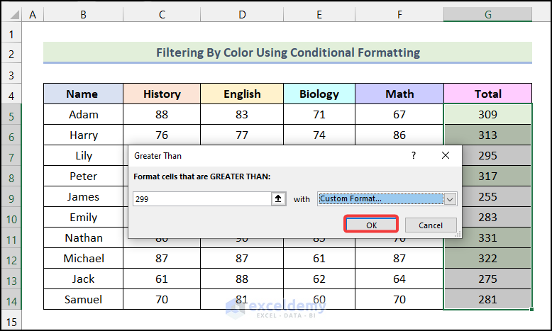
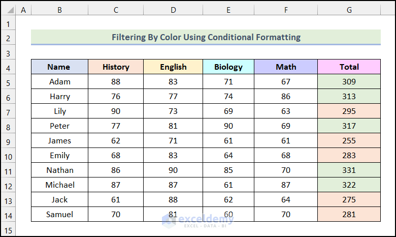
Consequently, you will have the cells formatted with your preferred color as shown in the following picture.

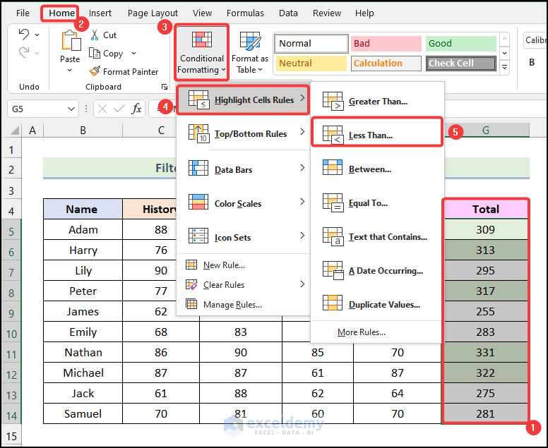
• Now, select the cells of the Total column as marked in the following image.
• Next, go to the Home tab from Ribbon.
• Then, select the Conditional Formatting option from the Styles group.
• Following that, choose the Highlight Cells Rules option from the drop-down.
• Subsequently, click on the Less Than option.

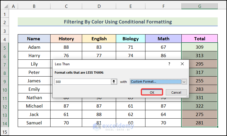
As a result, you will have the Less Than dialog box on your worksheet.

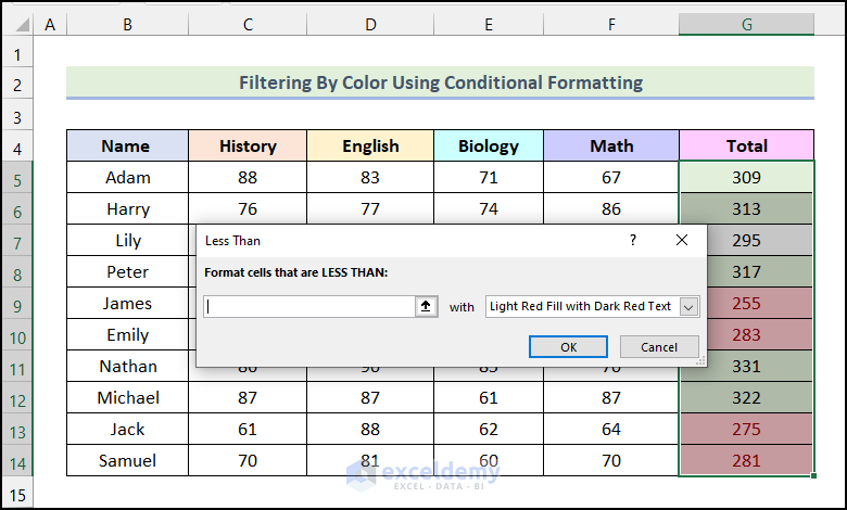
• Now, in the Less Than dialog box, type 300 in the marked field.
• After that, click on the drop-down icon and choose the Custom Format option from the drop-down.

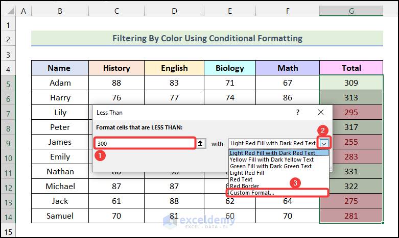
• Following that, in the Format Cells dialog box, go to the Fill tab.
• Next, choose your preferred color and click on OK.

• Subsequently, you will be redirected to the Less Than dialog box and click on OK.

Consequently, you will have the Total column formatted with your preferred colors.

Step 02: Enable Filter Option

At this stage, we will enable the Filter option. Let’s follow the steps given below.

• Firstly, select your data along with the headers.
• Then, go to the Data tab from Ribbon.
• Now, choose the Filter option from the Sort & Filter group.

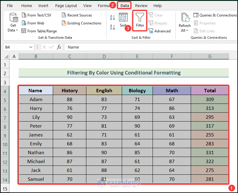
As a result, filtering options will be enabled as marked in the following image.

Note: You can also use the keyboard shortcut CTRL + SHIFT + L after selecting the data to enable the Filter option.

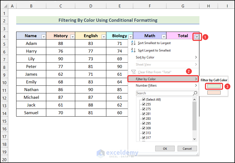
Step 03: Filter by Color

Now, we will filter our data based on the color of the cells. Follow the procedure mentioned below to do this.

• Firstly, click on the drop-down icon as marked in the following picture.
• Then, select the Filter by Color option from the drop-down.
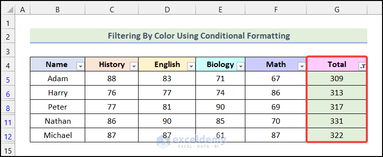
• After that, choose the color you want. Here, we chose the Green color.

Consequently, you will see the following output on your worksheet.

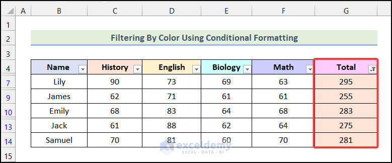
You can also choose the Red color and you will get the following output on your worksheet as shown in the following image.

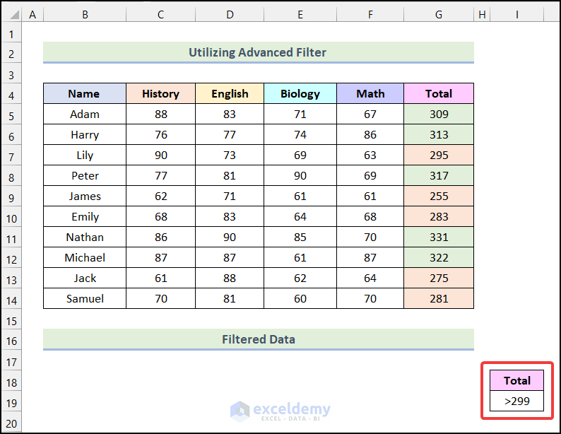
How to Use Advanced Filter Feature to Filter by Color in Excel

Advanced Filter is a quite handy feature of Excel. Using Advanced Filter, we can filter out data based on provided criteria within the same worksheet. Let’s say we want to filter our dataset based on 2 following criteria.

• Students who got more than 299 Total Marks.
• Students who got less than 300 Total Marks.

Let’s follow the steps mentioned below to filter our data by color using the Advanced Filter option.

Steps:

• Firstly, create a new column named Total and type in >299 in the cell below it.

Note: Here, the name of the newly created column must exactly match the Total column of the dataset.

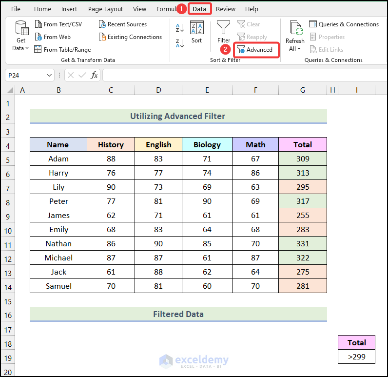
• Following that, go to the Data tab from Ribbon.
• After that, choose the Advanced option from the Sort & Filter group.

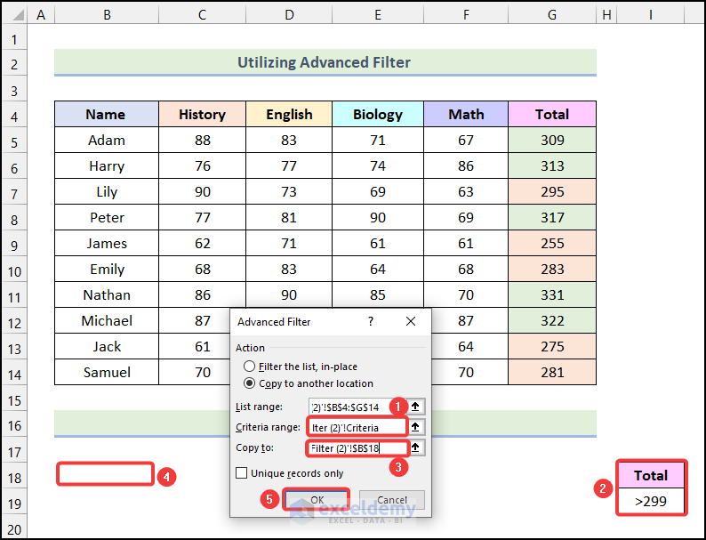
As a result, the Advanced Filter dialog box will open on your worksheet.

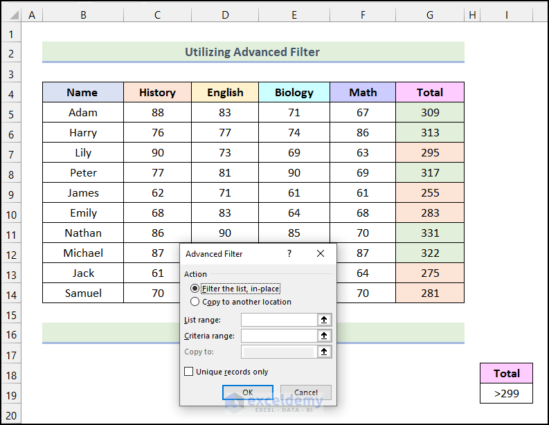
• Now, in the Advanced Filter dialog box, select the Copy to another location option under the Action field.
• Then, click on the List range field and select the dataset along with the headers as marked in the following picture.

• After that, click on the Criteria range field and choose the newly created column like in the image below.
• Next, click on the Copy to field and select cell B18. This is where your Filtered Data will be displayed.
• Finally, click on OK.

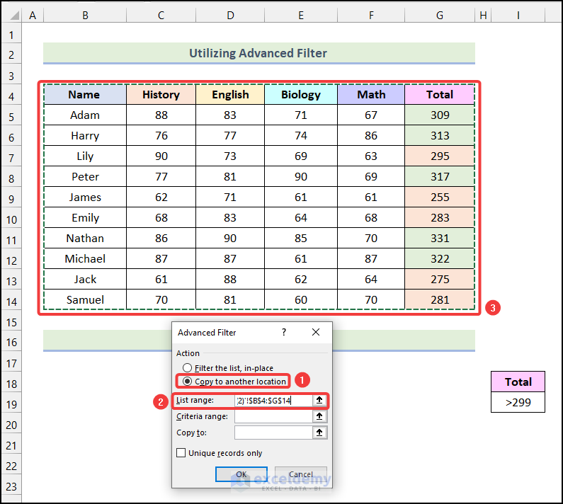
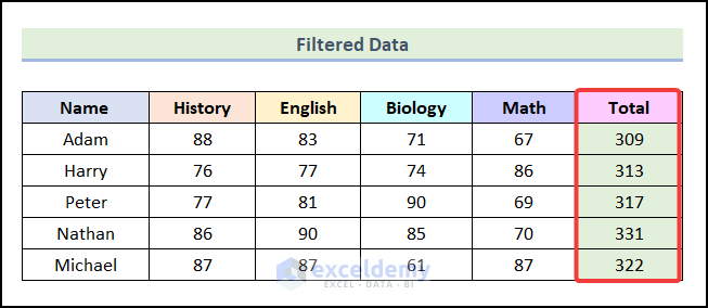
Consequently, you will have the list of students who got more than 299 Total Marks.

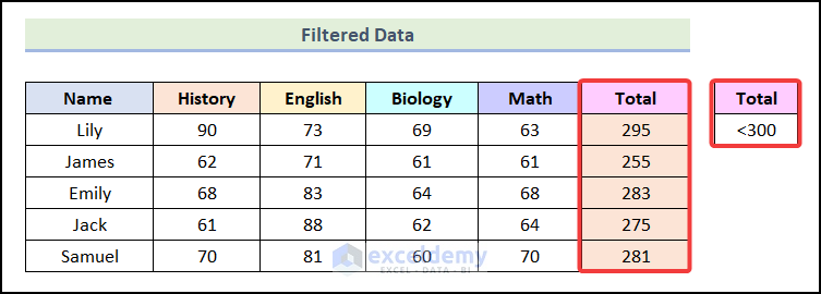
You can also change the condition to <300. By following the same steps, you will get the following output for the new condition as demonstrated in the following picture.

How to Solve If Filter by Color Option Is Not Showing in Excel

While working in Excel, sometimes we see that the Filter by Color option is not showing in Excel. In most cases, it happens when all the cells are formatted with the same color. Let’s say, we have the Marks of 10th Grade Students where all the cells of the Total column have a Yellow fill.

Let’s follow the steps mentioned below to solve the issue of the Filter by Color not showing.

Steps:

• Firstly, select the dataset along with the headers and go to the Data tab from Ribbon.
• Following that, choose the Filter option from the Sort & Filter group.

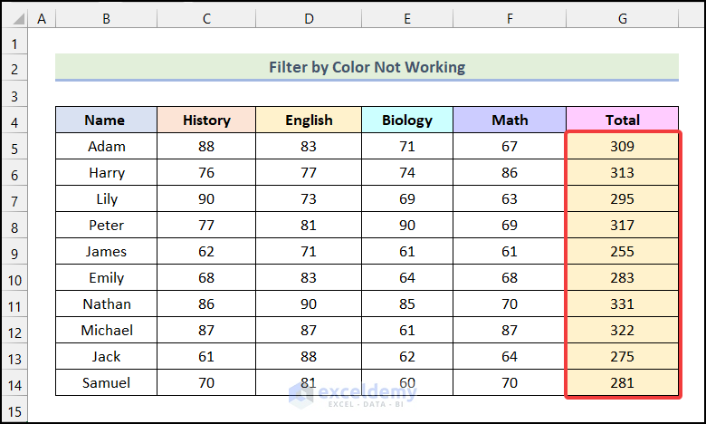
As a result, the options to filter will be added as shown in the image given below.

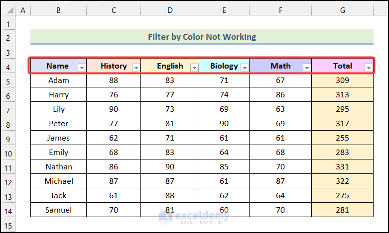
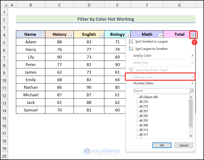
• Now, click on the drop-down icon beside the Total column.

You can see that the Filter by Color option is Grey. You can’t select it. Let’s solve this issue now.

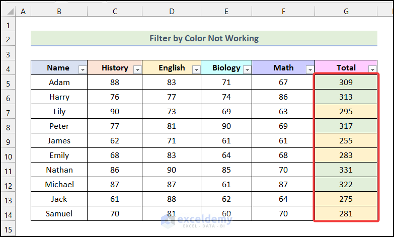
• Use the steps mentioned in Step 01 of the 1st method to apply conditional formatting to the dataset and get the following output.

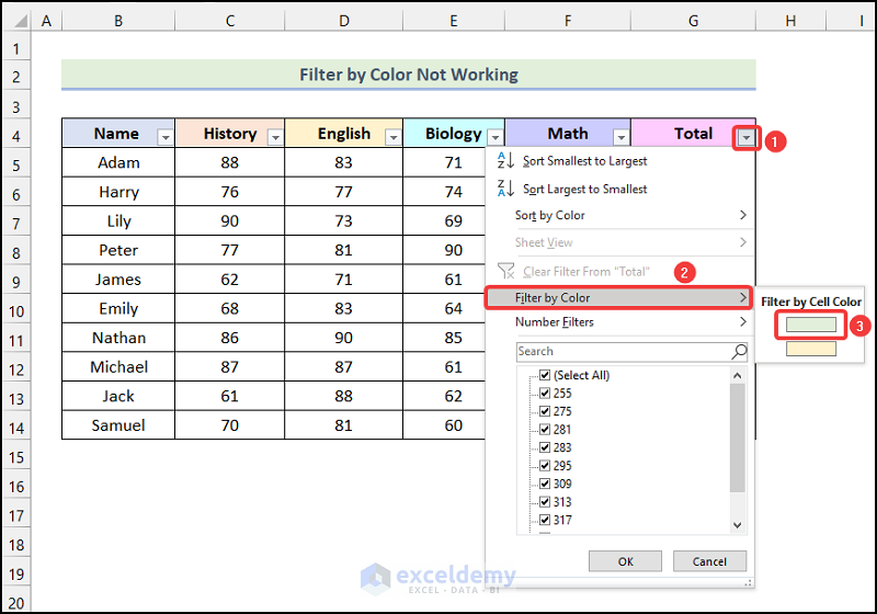
• Following that, click on the drop-down icon beside the Total column.
• Then, choose the Filter by Color option.
• Now, choose the color you want. In this case, we chose the Green color.

Subsequently, you will have the filtered output based on color as shown in the following image.

Download Practice Workbook

Conclusion

That’s all about today’s session. I strongly believe that this article was able to guide you to filter data by color that is formatted by conditional formatting in Excel. Please feel free to leave a comment if you have any queries or recommendations for improving the article’s quality.

<< Go Back to Color Filter | Filter in Excel | Learn Excel