In this article, we will demonstrate how to filter multiple columns by color in Excel, and how to filter data by multiple colors too.
Suppose we have the below dataset containing several people’s names and the cities in which they reside in columns B and C.
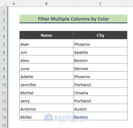
We’ll apply different colors to this dataset based on the data type, and then filter the data by color using two methods.
Method 1 – Using the Filter Feature to Filter Multiple Columns by Color
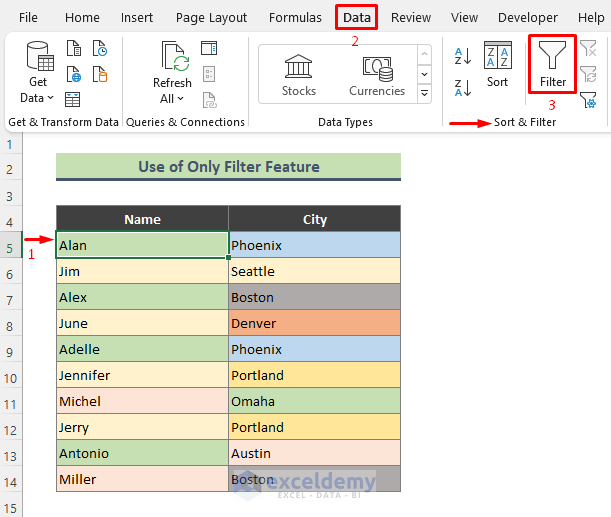
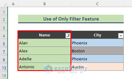
In this method, we’ll filter multiple columns by color using Excel’s regular Filter option only. In our dataset, names start with the letters A, J, and M. We’ve highlighted the cells in column B with different colors according to the first letter of the name. For instance, all the names starting with A are in green. Then we’ve highlighted duplicate cities in similar colors. For example, the city Phoenix is present twice, so both of the cells are blue.
Now we’ll filter column B by the color green, and column C by blue.

Steps:
- Select any cell in the dataset, then from the Ribbon go to Data > Filter. Or use Ctrl + Shift + L to apply the Filter.
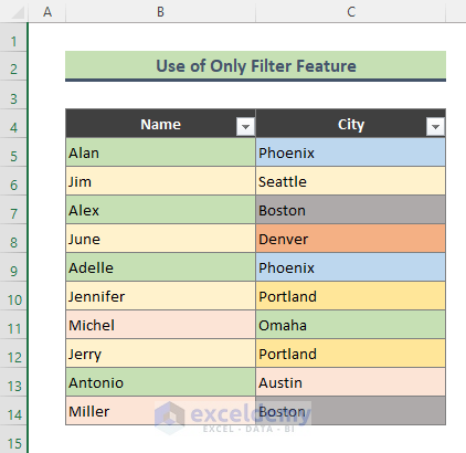
As a result, the drop-down arrow for the filter appears next to our Header cells..
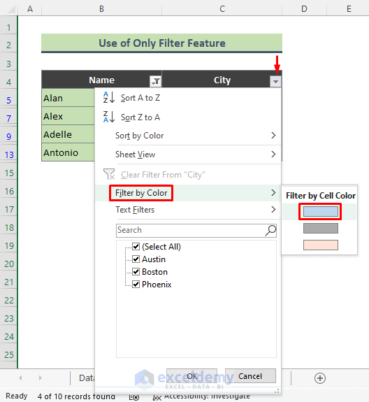
- Click on the dropdown arrow for column B, select Filter by Color, and choose green from Filter by Cell Color (as in the screenshot below).
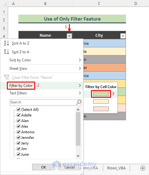
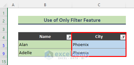
Column B is filtered by the color green.
Now we’ll filter column C by another color.
- Select the drop-down arrow, click on Filter by Color, and choose the color blue.
Column C is filtered by the color blue. So, we have successfully filtered multiple columns by color.
Method 2 – Using Excel VBA to Filter Multiple Columns by Color
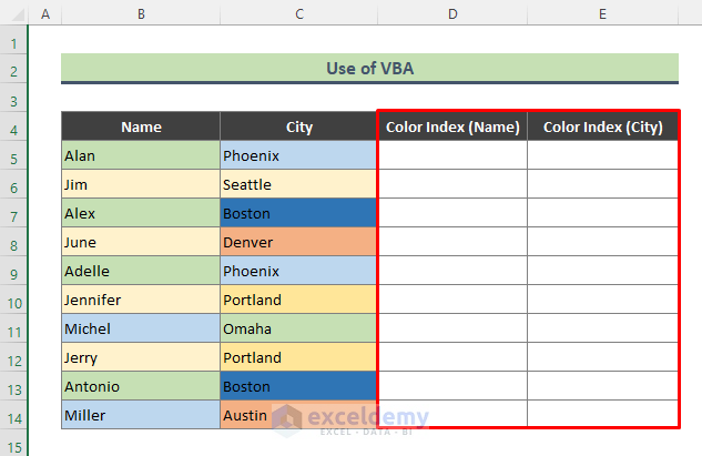
Now we’ll use a simple VBA code to create a User Defined function to find the color index for each color applied to the cells of columns B and C. Then we’ll filter column B for names starting with J (in the peach color) and column C for the city Portland (light orange color).
Steps:
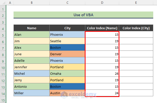
- Add two helper columns to the original dataset as follows:
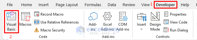
- To create a UDF, go to Developer > Visual Basic to open the VBA window (or press Alt + F11).
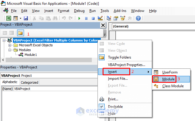
- In the VBA window, right-click on the VBAProject and go to Insert > Module.
- Enter the following code in the Module:
Function FindColor(n As Range) As Integer
FindColor = n.Interior.ColorIndex
End Function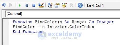
- Go to the worksheet where the newly created function will be applied.
- Enter the below formula in Cell D5, and press Enter:
=FindColor(B5)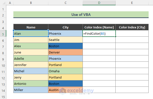
The color index of Cell B5 is returned.
- Use the Fill Handle (+) tool to get the color index for the rest of the colored cells in column B.
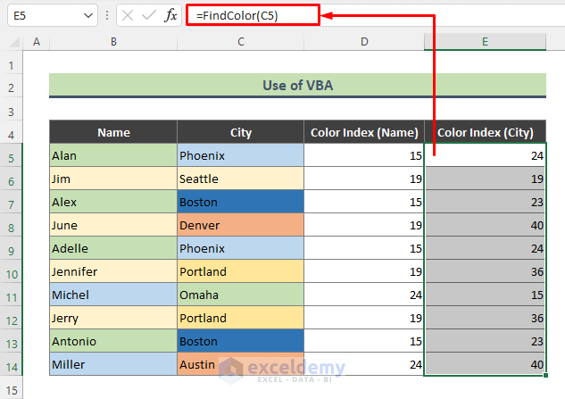
- Similarly, use the same function to get the color index of the cities in column C.
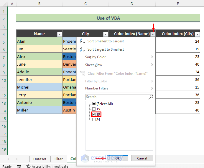
- Apply the Filter to the dataset by pressing Ctrl + Shift + L.
- Click on the filter drop-down arrow of column D and add a checkmark only for the color index 19.
- Click OK.
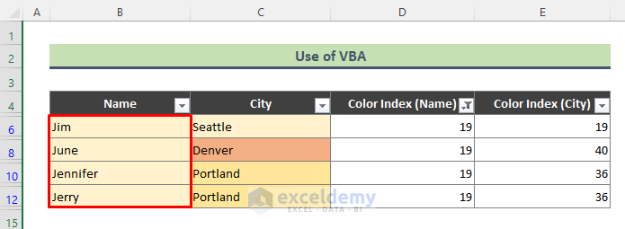
The below output is returned. As we have filtered column C only for peach color (index: 19), column B is also filtered for the same color, which applies to names starting with the letter J.
- Similarly, filter column E for color index 36.
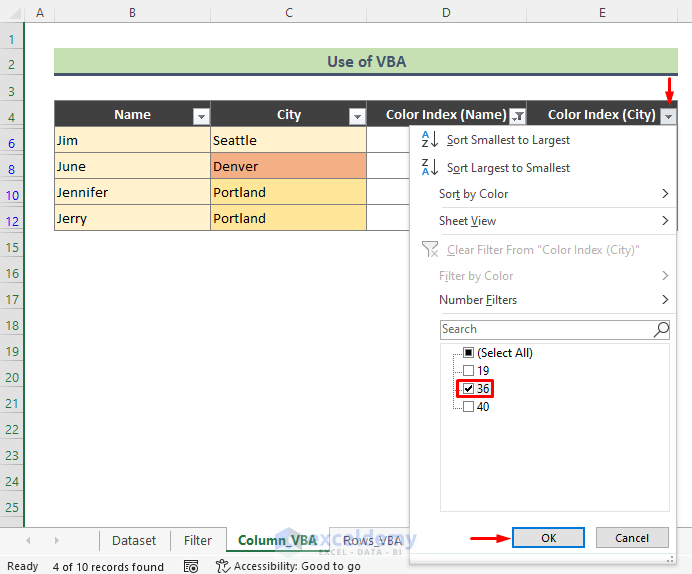
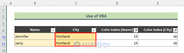
When column E is filtered for color index 36, column C is filtered for the light orange color which applies to the city of Portland.
So, we have successfully filtered multiple columns (columns B and C) by color.
How to Filter Data by Multiple Colors in Excel
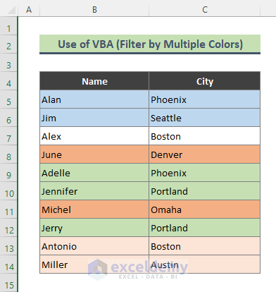
Usually in Excel we filter data by one color only, but we can filter rows or a column by multiple colors too with a VBA UDF. Suppose we have highlighted the rows of the below dataset in different colors. Now we will filter the rows by the colors green and blue.
Steps:
First, create the VBA UDF to find the color index.
- Press Alt + F11 to bring up the VBA window.
- Insert a Module from VBAProject as in Method 2.
- In the new Module, enter the same VBA code used in Method 2.
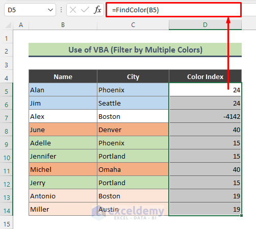
- Insert a helper column next to the original data.
- Enter the below formula in Cell D5 and press Enter:
=FindColor(B5)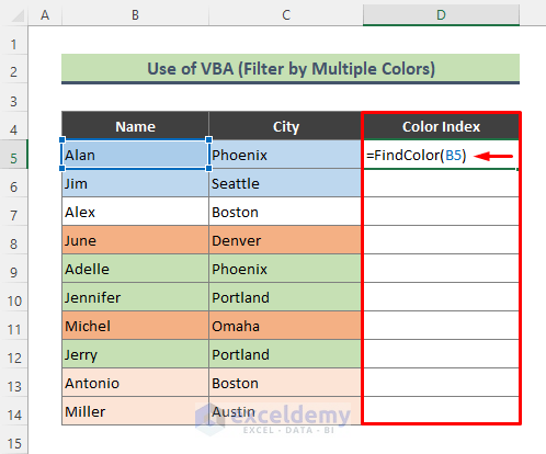
The color indices for all colors present in the rows below are returned.
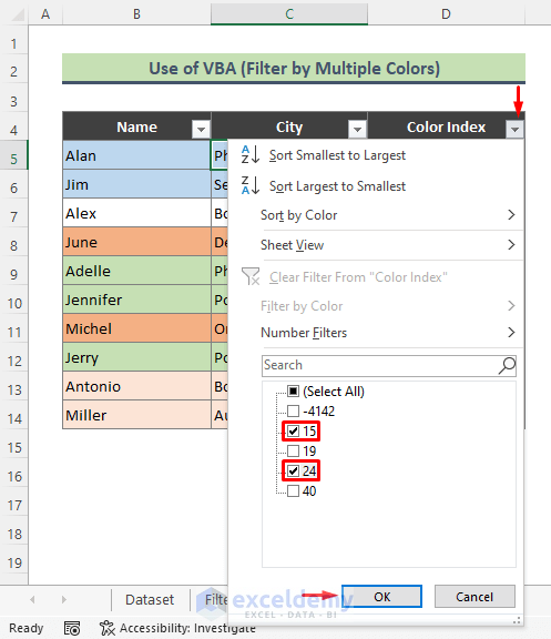
- Apply the Filter to the dataset.
- Click on the drop-down icon of column D, and place a checkmark only on the indices 15 and 24.
- Click OK.
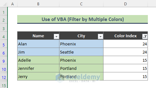
The dataset is filtered for rows colored in blue and green.
We have successfully filtered rows by multiple colors (blue and green) at the same time.
Download Practice Workbook
<< Go Back to Color Filter | Filter in Excel | Learn Excel
Get FREE Advanced Excel Exercises with Solutions!
