Excel Filter by Color and Text (with Easy Steps)

This article illustrates how to filter by color and text in Excel. You can easily filter by color text in Excel. But there is no direct way to do that by both criteria together. We will show you a way around doing that in this article. The steps are quick and easy to follow. So have a quick look through the article.

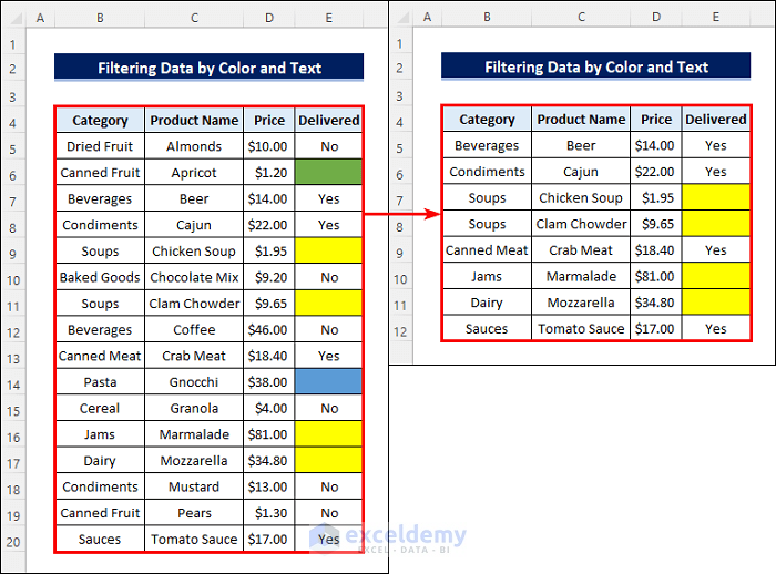
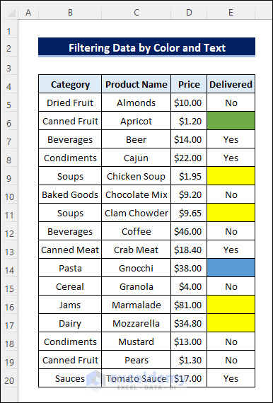
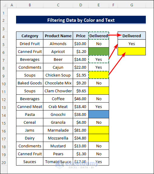
Assume you have the following dataset. Here the colored cells are blank. You want to filter the dataset by the “Yellow” cell color and the ” Yes ” text in column E.

We can not do that using the simple Filter command. So we will use Advanced Filter to get the desired result. Make a copy of your dataset and then follow the steps below to do that.

STEP 1: Replacing Values of Colored Cells to Filter by Color and Text

• First, select the data range or the colored cells. Then press CTRL + H to open the Find & Replace dialog box. Make sure you are in the Replace tab. Now click on the Format dropdown arrow for the Find what box. Then select “Choose Format From Cell”.

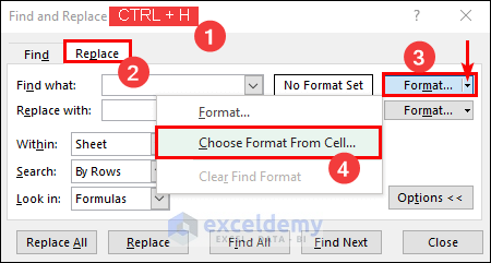
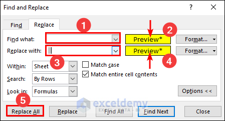
• Next, click on a yellow-colored cell. The format preview will change accordingly. Now enter a space in the “Replace with” Then pick the same cell color formatting as earlier. After that, select Replace All >> OK >> Close.

STEP 2: Setting Criteria for Advanced Filter

• Now copy the column header, a cell each from the cells with the desired color and the cells with the desired text. Then paste the cells on cell G4.

STEP 3: Applying Advanced Filter

• Now select the cell where you want to get the filtered data.

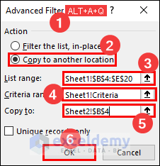
• Then press ALT + A + Q to apply the Advanced Filter. You can also do that from the Data tab. Next, mark the radio button for “Copy to another location” in the Advanced Filter dialog box. Then select the entire dataset as the List Range. Next, select the cells in column G as the Criteria range. After that, select the location where you want to get the filtered data and then click OK.

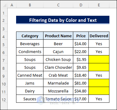
• Finally, you will get the following result.

Things to Remember

• You can not use blank cells as the filter criteria. That’s why you need to replace the blank colored cells with a space.
• Don’t set the filter criteria manually. Rather copy the desired cells from the dataset and paste them into the criteria range.
• Make a copy of your dataset to avoid any data loss while using the replace command.

Download Practice Workbook

You can download the practice workbook from the download button below.

Conclusion

Now you know how to filter by color and text in Excel. Is this what you need? You can let us know in the comment section below. Please share your queries or suggestions too.

<< Go Back to Color Filter | Filter in Excel | Learn Excel