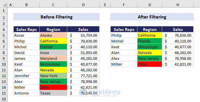
Consider the following data showing the sales information of some representatives from different regions. Here’s an overview of filtering data by multiple colors (yellow, green, and red) in the Region column.
2 Ways to Filter by Multiple Colors in Excel
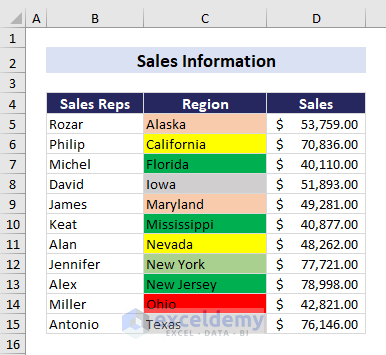
Let’s say we have a dataset containing several sales representatives’ names, their regions of sales, and sales amounts in columns B, C, and E, respectively. The Region column has different colors for different regions. We will filter the data by multiple colors (yellow, green, and red) in the Region column.
Case 1 – Using the Color Code
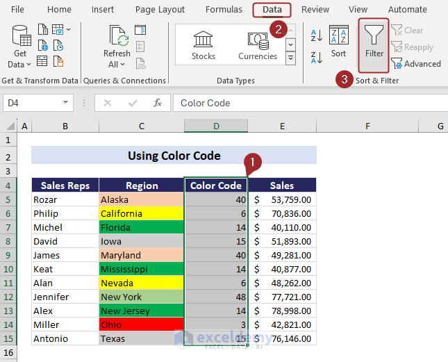
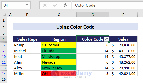
Let’s say, we have the code of each color used in the Region column. For the data below, we will filter our data by multiple colors using the color code with the Filter feature. The code for red is 3, for yellow 6, and for green 14.
- Select any cell.
- Go to the Data tab and Sort & Filter group, then choose Filter.
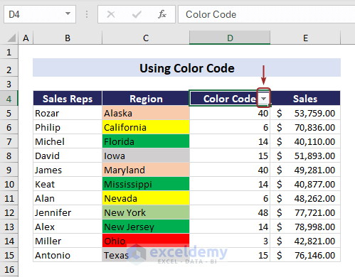
- The drop-down arrow for the filter appears in the heading.
- Click on the drop-down arrow in the column with the color code.
- Select the code of your desired color and click OK.
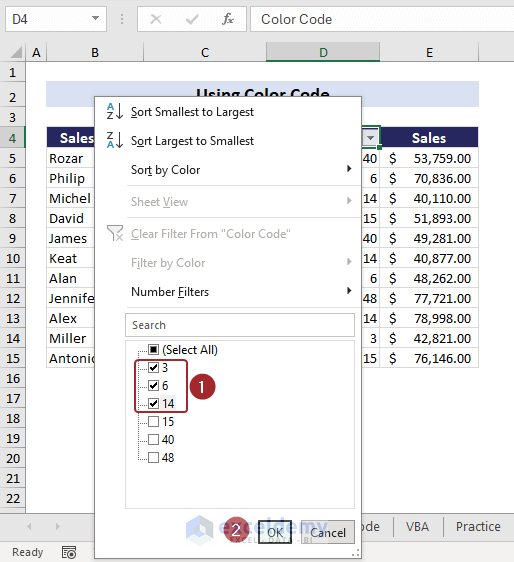
- You will be able to filter by multiple colors using the color code.
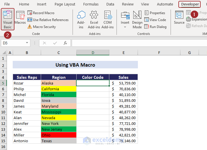
Case 2 – Using VBA Macro
- Go to the Developer tab and select Visual Basic or press Alt + F11.
- The Microsoft Visual Basic for Applications window will appear.
- Click on Insert and Module.
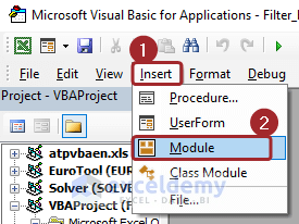
- This will launch a Module window.
- Insert the following code in the Module:
Function FindColor(n As Range) As Integer
FindColor = n.Interior.ColorIndex
End Function- You don’t need to run the code. This will automatically create a function called FindColor.
- Switch back to the Excel worksheet.
- Select a cell and apply the formula:
=FindColor(D5)
Here, cell D5 contains the color.
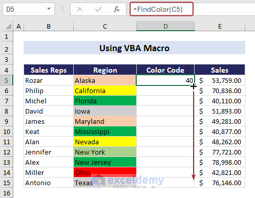
- Drag the Fill handle to copy the formula down.
- You will get the color code or color index for all the colors in the column.
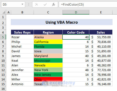
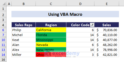
- Use the color code section above to filter data by multiple colors in Excel.
Download the Practice Workbook
Frequently Asked Questions
How to select all colored cells in Excel?
To select all colored cells in Excel, follow these steps:
- Navigate to the “Home” tab > “Editing” group >”Find & Select“.
- Click on “Go To Special” from the dropdown menu.
- In the “Go To Special” dialog box, choose “Constants” and “Fill Color.”
- Pick the specific color or leave it as “Any Fill” to select all colored cells.
- Click “OK” to apply the selection.
How to sort multiple cells by color in Excel?
To sort multiple cells by color in Excel:
- Highlight the cells you want to sort.
- Go to the “Data” tab > “Sort” to open the Sort dialog box.
- Select the column and sorting order as usual.
- Click “Add Level“.
- Choose “Sort On” > “Cell Color.”
- Pick the cell color for sorting and set the order.
- Add more levels for additional color sorting.
- Click “OK” to apply the sorting based on color.
How do I remove color filters in Excel?
To remove color filters, go to the “Data” tab and turn off “Filter” button. It will remove the color filter and switch back to the original data.
<< Go Back to Color Filter | Filter in Excel | Learn Excel
Get FREE Advanced Excel Exercises with Solutions!
