Sample Excel File with Employee Data for Practice

In this example, you will get a sample Excel file with employee data for practice. The problems are beginner-friendly and you will need to know the following features and functions: how to join two cell values, the Data Validation list, the VLOOKUP, and the IF functions. These features and functions are available from Excel 2007.

Download the Practice Workbook

Problem Overview

We have an Excel dataset with six columns for employee information. The first two columns are filled in. You will fill in the rest of the values in the dataset as per instructions. We have set today’s date in cell B28 to calculate date-related values.

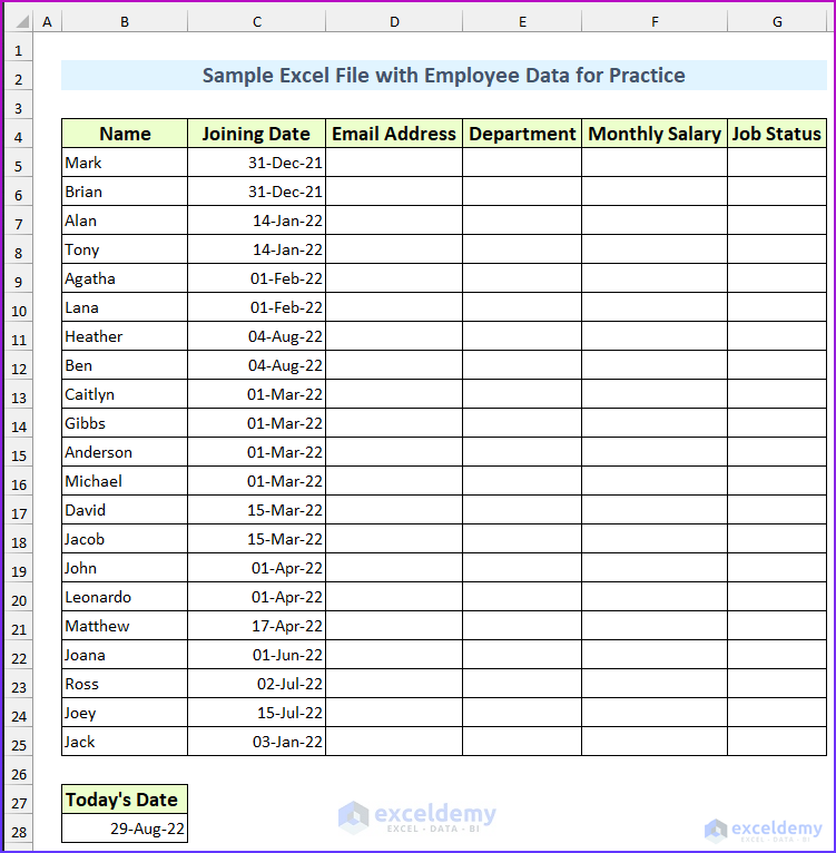
Here’s how to fill the rest of the information.

• Email Address – The format will be “[email protected]”.
  • Solution: We have used the ampersand operator to join the values from the Name column with the email domain. You can use other methods, such as the CONCATENATE, TEXTJOIN functions, or even VBA to do so.

• Department – You will need to create a Data Validation in this column. This Excel feature helps us to restrict data entry. The source for data validation is on the “Reference Table” Sheet (Range B5:B11).

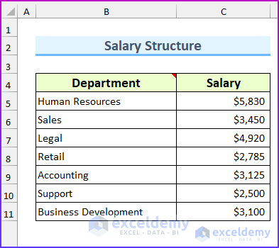
• Salary –  There is a lookup table in the “Reference Table” Sheet. Your task will be to match the department name and return the monthly salary in that. You can use any lookup function to do so.
  • Solution: We have used the VLOOKUP function to solve this problem. However, you can also use any other lookup function to do so, such as the INDEX, MATCH, XLOOKUP functions.

The lookup table looks like this.

• Job Status – If an employee joined more than 180 days ago, they will be a permanent employee of the company. You need to use conditionals to solve this.

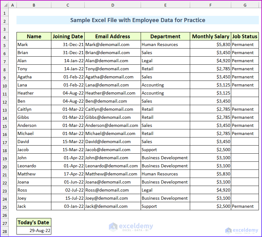
The completed Excel file will look similar to this.