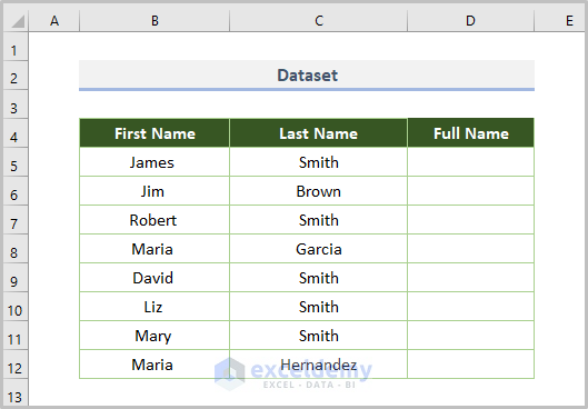
We’ll use the following dataset, with a list of first and last names. We’ll merge those into full names in column D.
Method 1 – Merging Text with the Ampersand Symbol (&)
Case 1 – Ampersand Symbol without Separator
- Insert the following formula in D5:
=B5&C5
B5 is the starting cell of the first name and C5 is the starting cell of the last name from the dataset.
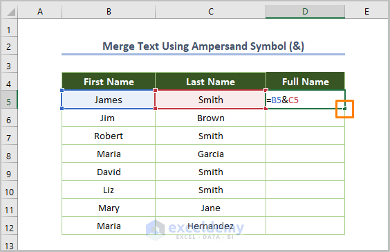
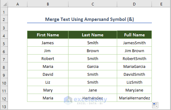
- Hit Enter and drag the Fill Handle from D5 down to fill the rest of the column.
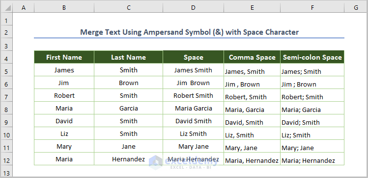
Case 2 – Ampersand Symbol with a Delimiter
- Use the following formula in D5:
=B5&" "&C5
We put space inside double quotes to include the space between the first and last name.
- If you need to use comma space, input the comma instead of the space.
=B5&", "&C5
- You can also use the semicolon and a space:
=B5&"; "&C5
However you decide to separate the first from the last name, just insert your desired delimiters between double quotes as an argument for the ampersand operator.
- After entering the formula and using the Fill Handle Tool, our output will be as follows.
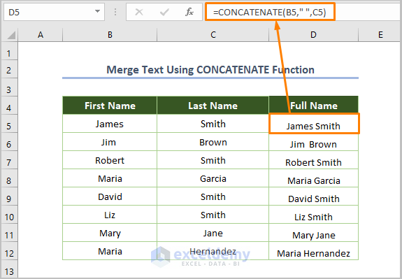
Method 2 – Combining Text with the CONCATENATE Function
- Use the following function in cell D5:
=CONCATENATE(B5," ",C5)
Here, B5 is the starting cell of the first name and C5 is the starting cell of the last name. We inserted a space between them.
- Press Enter and use the Fill Handle Tool.
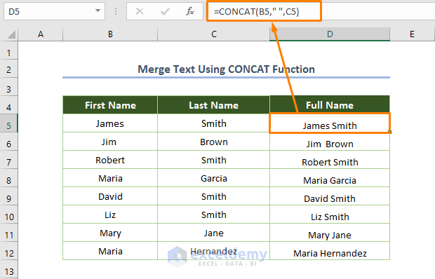
Method 3 – Joining Text with the CONCAT Function
The CONCAT function is a newer version of CONCATENATE.
- Use the following formula in D5:
=CONCAT(B5," ",C5)
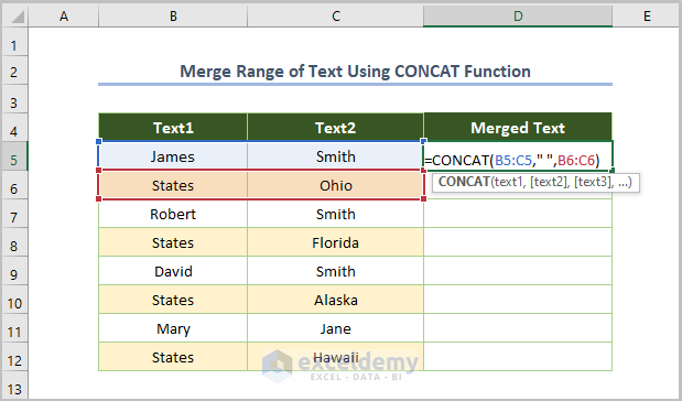
The CONCAT function can also combine a range of cells.
Here’s an example of the formula with arrays as string arguments.
=CONCAT(B5:C5," ",B6:C6)
B5 and C5 are the cells with the first names but B6 and C6 are the cells for respective last names. The function will work sequentially, concatenating all cells from one array, then go to the next argument.
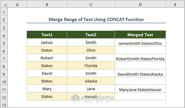
Here’s the output for the array example when AutoFilled.
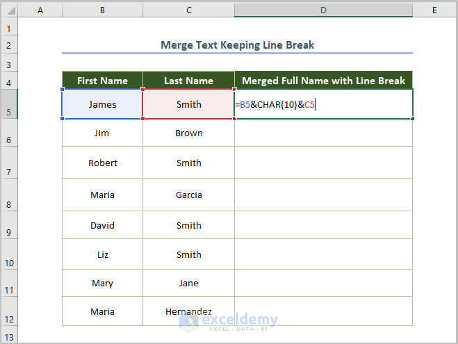
Method 4 – Merging Text with Line Breaks
- Use the following function in D5:
=B5&CHAR(10)&C5
Here, B5 is the starting cell of the first name and C5 is the starting cell of the last name. CHAR(10) is the code for a line break.
- Press Enter and use the Fill Handle tool to copy the formula throughout the column.

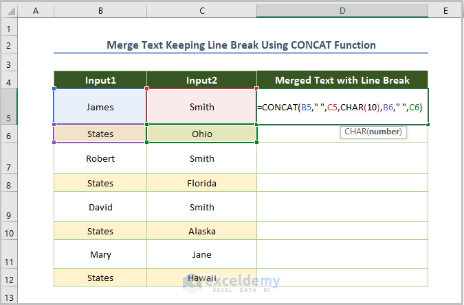
You can also use the CONCAT function to embed line breaks and spaces:
=CONCAT(B5," ",C5,CHAR(10),B6," ",C6)
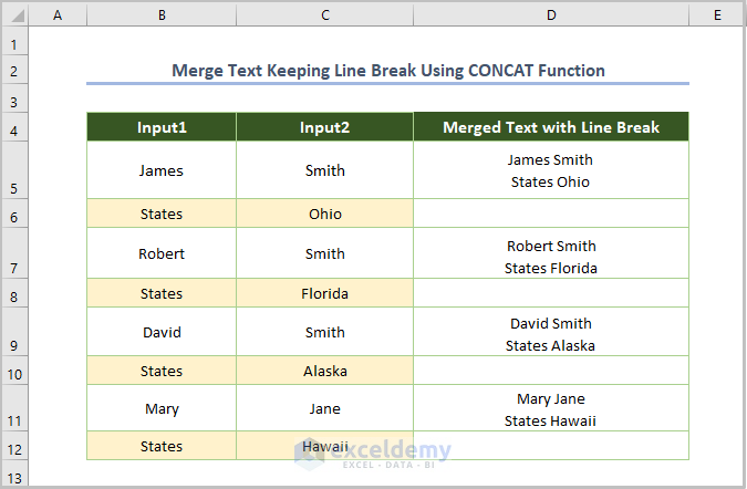
If you press Enter and use the same formula except changing the cell name, you’ll get the following output.
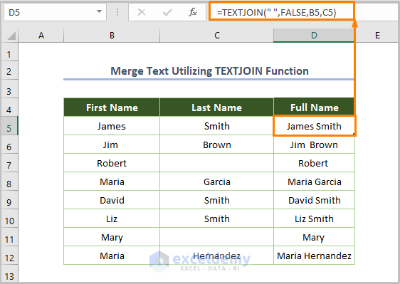
Method 5 – Merging Text from Two Cells with the TEXTJOIN Function
The TEXTJOIN function is available from Excel 2019.
- Use the following formula in D5:
=TEXTJOIN(" ",FALSE,B5,C5)
B5 is the starting cell of the first name and C5 is the starting cell of the last name. We put FALSE as the second argument to ensure that the formula doesn’t skip blank cells.
- Press Enter and use the Fill Handle to copy the formula throughout the column.
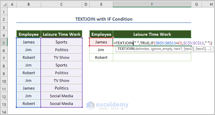
You can also use TEXTJOIN to merge text with conditions.
Consider a list of Leisure Time Work for some employees. We’ll list all the leisure activities for a particular employee.
- Use the following formula in cell F5 to fetch the leisure activities of the employee named in E5:
=TEXTJOIN(" ",TRUE,IF($B$5:$B$13=E5,$C$5:$C$13," "))
Here, “ “ is the delimiter, and TRUE is used to ignore blank cells. We used $B$5:$B$13=E5 as an array to assign the selected employee from the list of employees and $C$5:$C$13 to find the work for the selected employee.
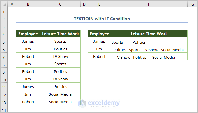
- Since this is an array function, press Ctrl + Shift + Enter to get the output.
- Use the Fill Handle Tool to copy the formula throughout the column.
Method 6 – Combining Text Using Power Query
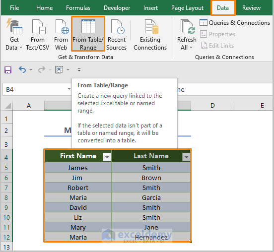
Step 1 – Inserting the Dataset into the Power Query Editor
- Select the entire dataset.
- Go to the Data tab.
- Select From Table/Range from the Get & Transform Data ribbon.
- If you get the Create Table dialog box, check My Table has headers and hit OK.
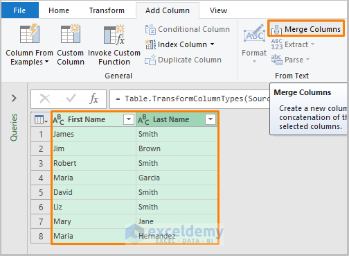
Step 2 – Merging the Columns
- You’ll get the Power Query Editor.
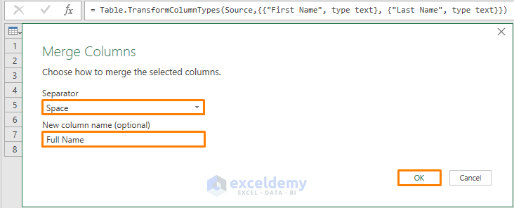
- Select the two columns by pressing Shift, then select Merge Column from the Add Column tab.
- For Separator, choose Space.
- Type Full Name in the blank space under New Column name.
- Press OK.
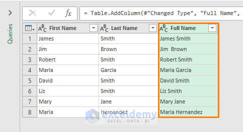
- You’ll get the following output with the full names.
Step 3 – Loading the Output into Worksheets
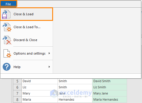
- Click File and select Close & Load.
- You’ll get an export dialog box. Select the cell or worksheet where you want the data and confirm.
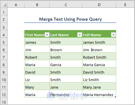
- Here’s the result.
Method 7 – Merging Text from Two Cells Using VBA
Steps:
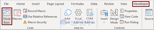
- Open the VBA window by going to the Developer tab and selecting Visual Basic.
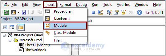
- Go to Insert and select Module.
- Paste the following code into the newly created module.
Sub MergeText_VBA()
    Dim SourceCells As Range
    Dim DestinationCell As Range

    Set SourceCells = Application.InputBox(prompt:="Select the cells to merge", Type:=8)
    Set DestinationCell = Application.InputBox(prompt:="Select the output cell", Type:=8)
    temp = ""
    For Each Rng In SourceCells
        temp = temp & Rng.Value & " "
    Next
    DestinationCell.Value = temp
End Sub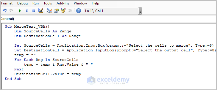
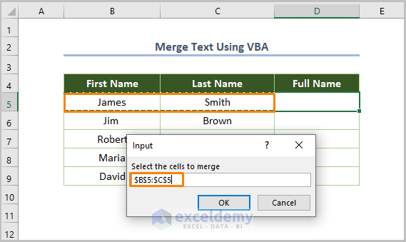
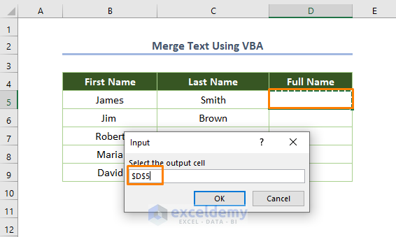
- Run the code (the keyboard shortcut is F5 or Fn + F5), and you’ll see the following dialog box where you have to select the cells that you want to merge.
- You’ll get the following dialog box to choose the destination cell where you want to get the merged text.
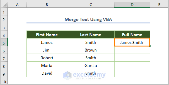
- You’ll get the merged text as shown in the below.
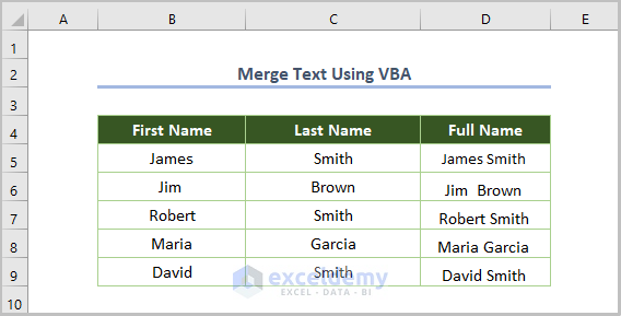
- Repeat the process for all cells.
Download the Practice Workbook
<< Go Back to Concatenate Excel | Learn Excel
Get FREE Advanced Excel Exercises with Solutions!

ALHAMDULILLAH, JAZAQHALLA
Hello Athikula,
You are most welcome. Keep exploring Excel with ExcelDemy!
Regards
ExcelDemy