How to Merge Cells Using Excel Formula (8 Formulas)

Formula 1 – Merging Multiple Cells Using the Merge & Center Feature in Excel

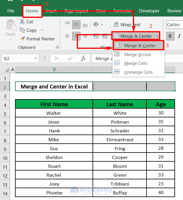
The dataset has a text “Merge and Center in Excel” in cell B2. We will merge it with the adjacent C2 and D2 cells in the same row. The three cells will be merged into one and the text will cover the entire area of these 3 cells (B2, C2, D2).

Step 1:

Select the 3 cells to merge (B2, C2, D2).
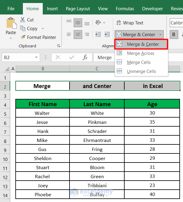
Go to the Merge and Center drop-down menu in the Alignment section under the Home tab.
On clicking the Merge and Center drop-down menu, you will see a list of different types of merge options. Select Merge and Center.

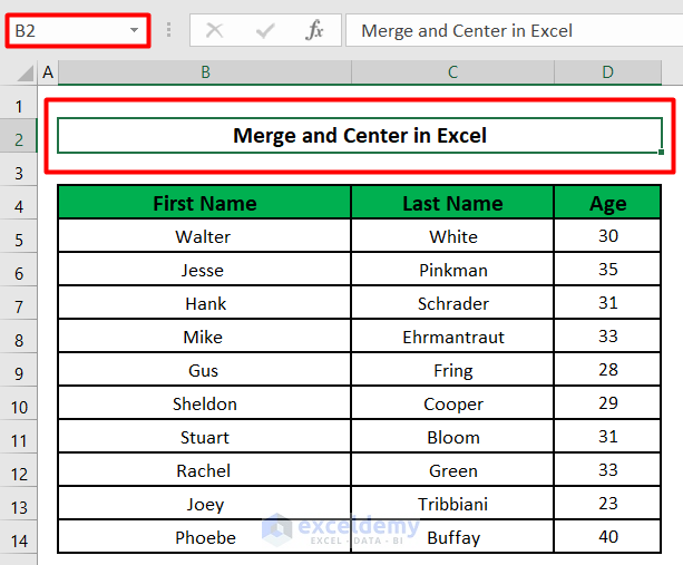
The three cells will be merged into one cell. The address of the merged cell is B2. The text now covers the space of all 3 cells.

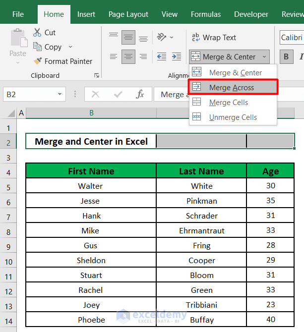
Step 2:

We can also try the other merge options from the Merge and Center drop-down menu. The Merge Across option will merge the selected cells in the same row into one large cell.

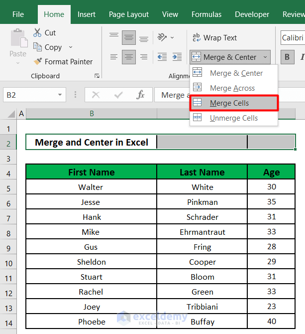
The merge Cells option will merge the selected cells into one cell but it will not center align the content of the cells in the new merged cell.

Formula 2 – Combining Multiple Cells with Contents Using Merge and Center

Step 1:

Select the Merge and Center option from the Merge and Center drop-down menu.

Step 2:

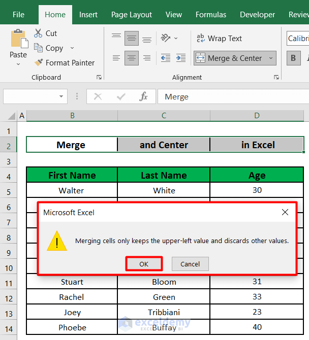
A warning dialog box will appear that will tell you that merging cells will only keep the content of the upper-left value while discarding the contents of the rest of the cells. In this example, merging cells will only keep the content or text of cell B2 (“Merge”) and remove the contents of the rest of the cells (C2, D2).
Click on OK.

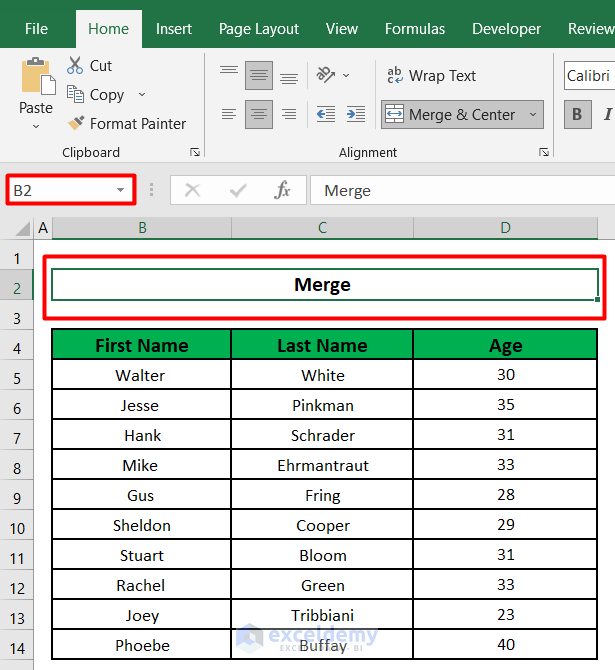
The 3 cells will be merged into one large cell with the cell address B2. But it contains only the text of cell B2 (“Merge”) before merging.

Formula 3 – Using Ampersand Symbol (&) to Merge Multiple Cells in Excel

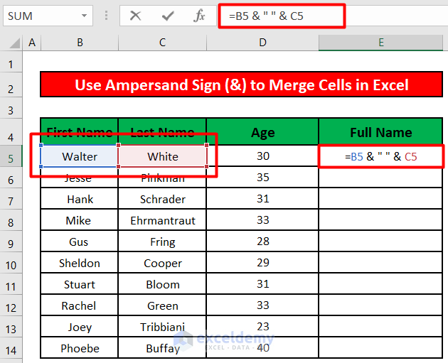
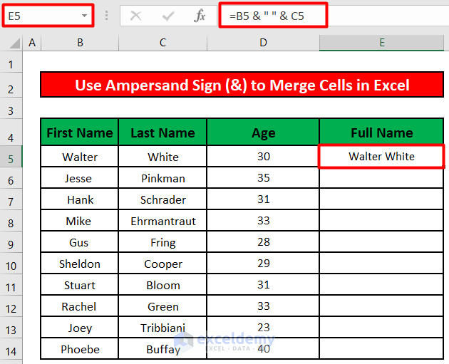
We will combine the First Name in cell B5 and the Last Name in cell C5 using the ampersand symbol (&) to generate the Full Name.

Step 1:

Enter the following formula in cell E5.

=B5 & " " & C5

Formula Breakdown:

The two ampersand symbols (&) will join the text in cell B5, space (“ ”), and text in cell C5.

On pressing ENTER, you will see that cell E5 has now the Full Name of the first employee.

Step 2:

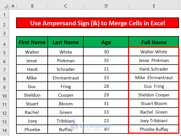
Drag the fill handle of cell E5 to apply the formula to the rest of the cells.

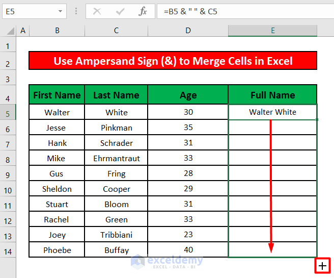
Each cell in the Full Name column will have the full name of the respective employee in that row.

Step 3:

We can also add additional text between the cells before joining them using the ampersand (&) symbol.
Enter the following formula in cell E5.

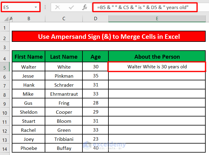
=B5 & " " & C5 & " is " & D5 & " years old"

Formula Breakdown:

The ampersand symbols (&) will join the text in cell B5, space (“ ”), text in cell C5, text in cell D5, and two additional strings: “is” and “years old”.

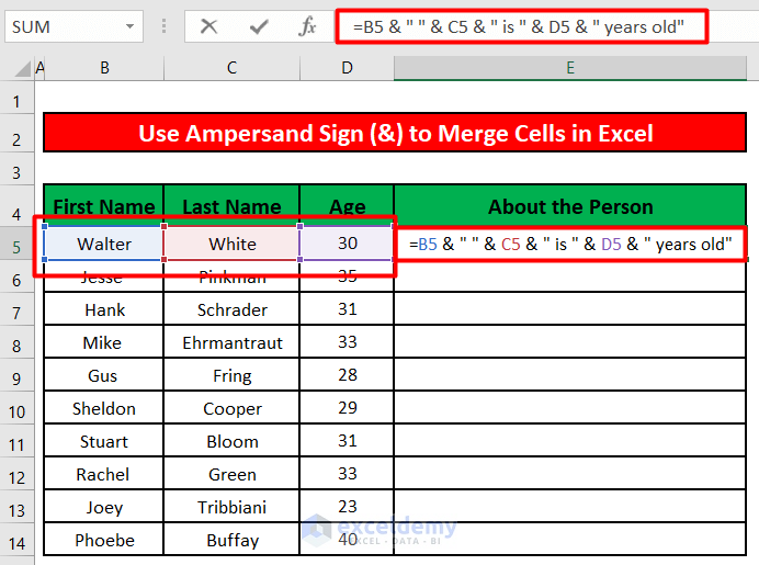
On pressing ENTER, cell E5 will have the following text in it: Walter White is 30 Years Old.

Step 2:

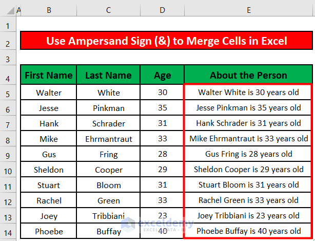
Drag the fill handle of cell E5 to apply the formula to the rest of the cells.

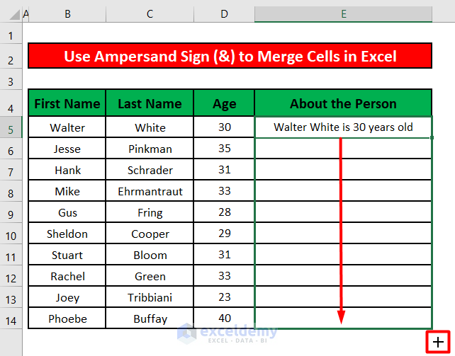
Each cell in the About the Person column will have a similar text.

Formula 4 – Applying the CONCATENATE Formula to Merge Cells in Excel

Step 1:

Enter the following formula in cell E5.

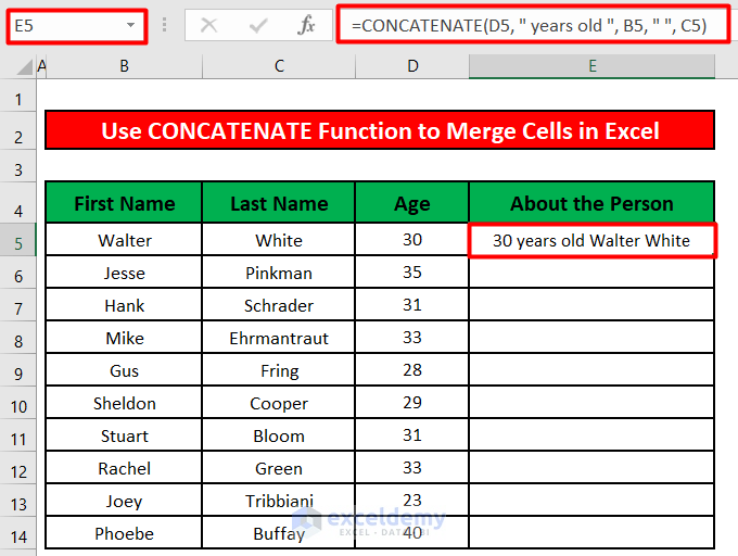
=CONCATENATE(D5, " years old ", B5, " ", C5)

Formula Breakdown:

The CONCATENATE formula takes 5 arguments.

The first one is the Age (D5).
The second argument is a piece of text “ years old ”.
The third argument is the First Name (B5) of the employee.
The fourth argument is a space (“ ”).
And the last one is the Last Name (C5) of the employee.

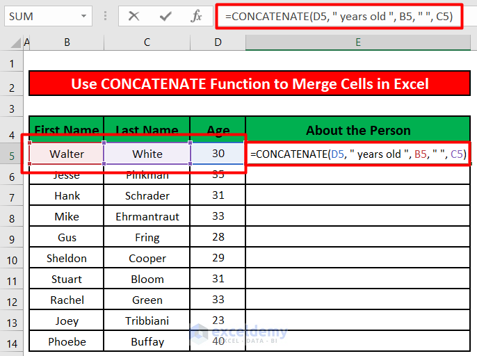
On pressing ENTER, cell E5 will have the following text in it: 30 Years Old Walter White.

Step 2:

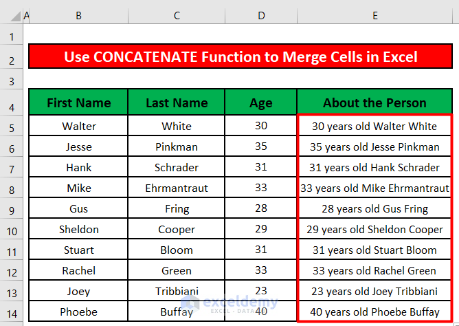
Drag the fill handle of cell E5 to apply the formula to the rest of the cells.

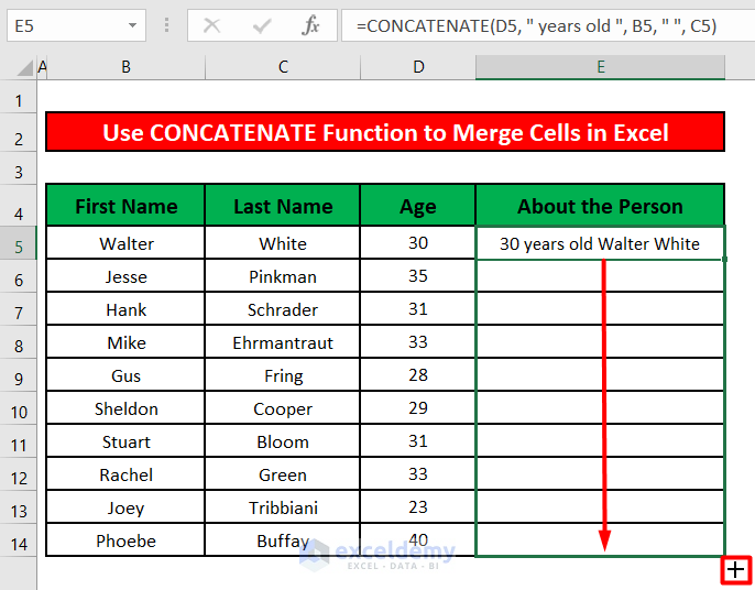
Each cell in the About the Person column will have a similar text.

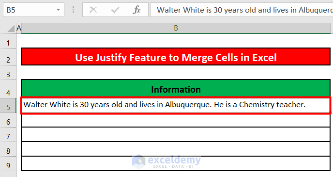
Formula 5 – Using the Justify Feature to Merge Cells in the Same Column

Step 1:

Select all the cells in the same column that we want to merge or combine.
Go to the Fill drop-down menu in the Editing section of the Home.
A new menu with different types of Fill options will appear. We will select Justify.

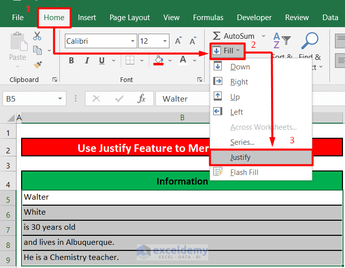
The texts in all the cells under the Information column will be merged into the first or top-most cell (B5).

Click on Merge and Center in the Alignment section of the Home.

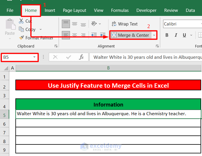
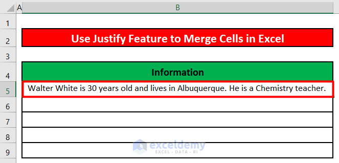
The merged text in the Information column will be centered in cell B5.

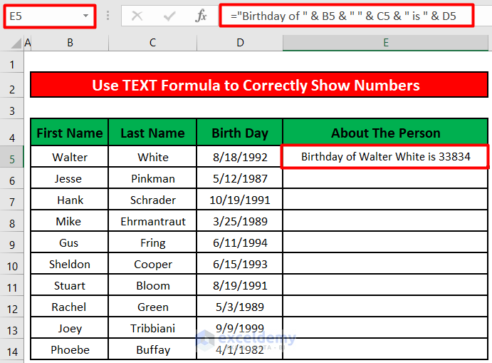
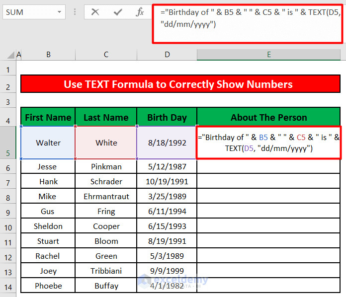
Formula 6 – Inserting the TEXT Formula in Excel to Correctly Display Numbers in Merged Cells

While using the ampersand (&) or CONCATENATE functions to merge cells in Excel, we will face a problem working the dates. As shown in the image below, the date values will be lost in the format due to merging of the cell values.

We can avoid this problem using the TEXT function in Excel.

Steps:

Enter the following formula in cell E5.

="Birthday of " & B5 & " " & C5 & " is " & TEXT(D5, "dd/mm/yyyy")

Formula Breakdown:

The TEXT function in Excel takes a value (D5) as the first argument and a text format (“dd/mm/yyyy”) as the second argument. It will return the text or the first augment in the text format that we have given it as the second argument.

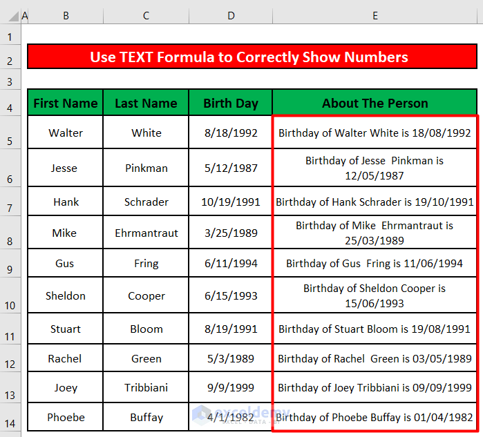
If we apply the formula to the rest of the cells in the About The Person column, we will see that the date values are now shown in the correct format.

Formula 7 – Finding Merged Cells Quickly Using Find and Replace Tool

Step 1:

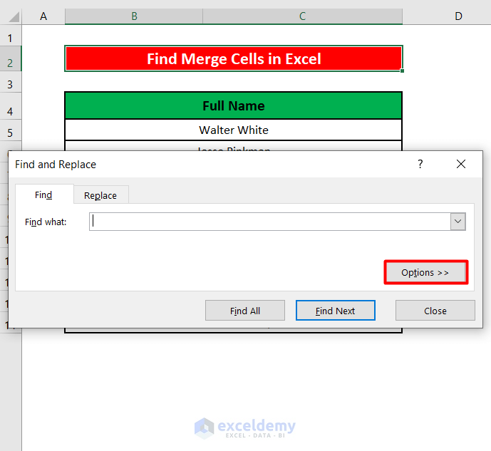
Press CTRL+F to activate the Find and Replace tool in Excel. A window titled Find and Replace will appear.
Click on the Options >>.

Step 2:

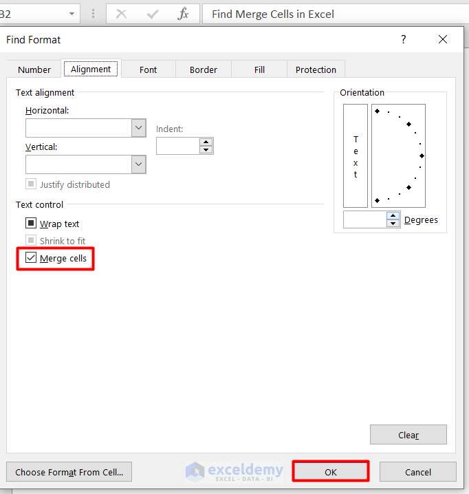
Click on the Format drop-down.

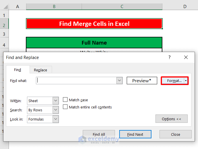
In the new window, click on the Alignment.
Check the box beside Merged cells.
Click on OK.

Step 3:

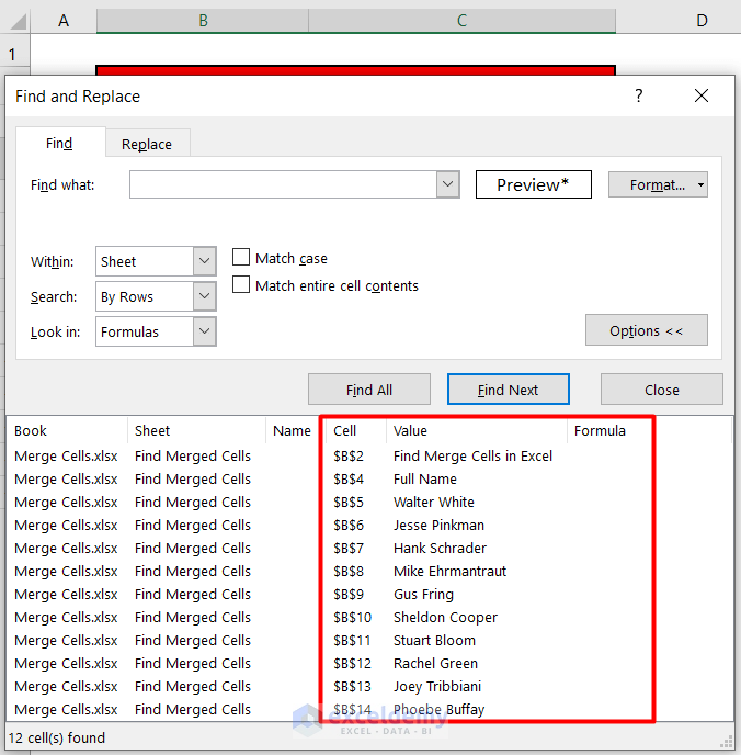
Click on the Find All button from the Find and Replace.

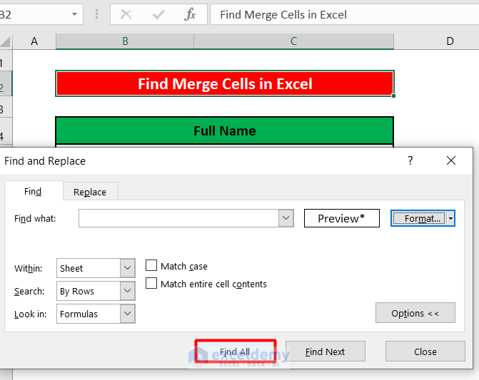
It will display all of the merged cells in the worksheet along with the cell addresses.

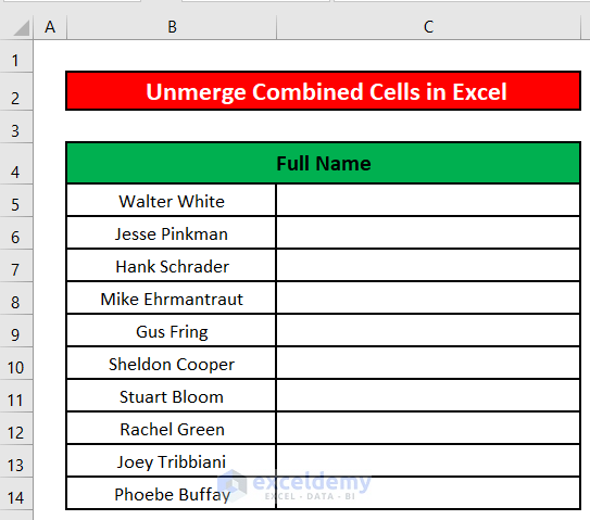
Formula 8 – Unmerging the Combined Cells in Excel

We can use the Unmerge Cells feature from the Merge and Center drop-down menu to unmerge the merged or combined cells in a worksheet.

Steps:

Select the merged cells. Go to the Merge and Center drop-down menu in the Alignment section under the Home.
On clicking the Merge and Center drop-down menu, you will see a list of different types of merge options. Click on the Unmerge Cells.

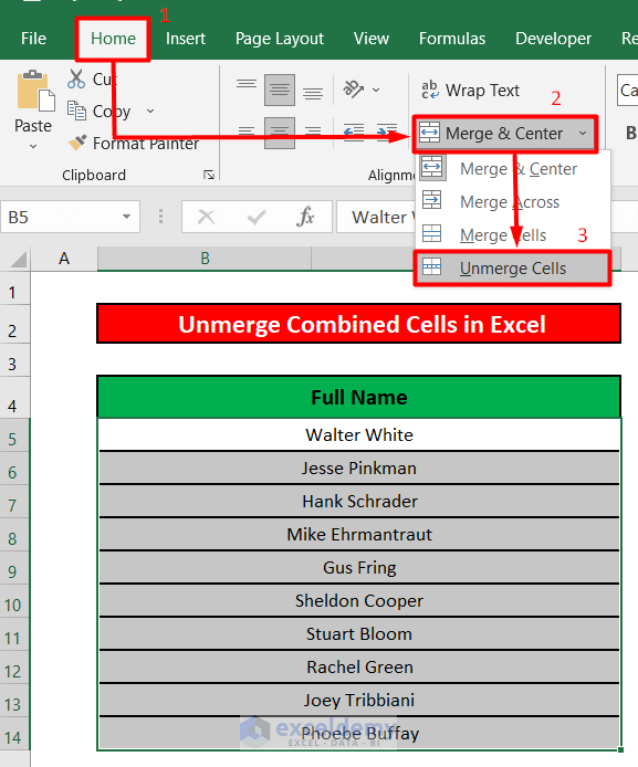
All the merged cells in the Full Name column will be unmerged.

Things to Remember

You can use keyboard shortcuts to merge cells.
- To activate the Merge Cells option: ALT H+M+M
- To Merge & Center: ALT H+M+C
- To Merge Across: ALT H+M+A
- To Unmerge Cells: ALT H+M+U
When merging multiple cells with text values, make a copy of the original data. Making a copy of the original data will prevent the risk of losing the data due to merging.